Exam 16: Regression Analysis: Model Building
Exam 1: Data and Statistics85 Questions
Exam 2: Descriptive Statistics: Tabular and Graphical Displays112 Questions
Exam 3: Descriptive Statistics: Numerical Measures139 Questions
Exam 4: Introduction to Probability129 Questions
Exam 5: Discrete Probability Distributions150 Questions
Exam 6: Continuous Probability Distributions144 Questions
Exam 7: Sampling and Sampling Distributions119 Questions
Exam 8: Interval Estimation118 Questions
Exam 9: Hypothesis Tests118 Questions
Exam 10: Inference About Means and Proportions With Two Populations127 Questions
Exam 11: Inferences About Population Variances113 Questions
Exam 12: Tests of Goodness of Fit, Independence and Multiple Proportions76 Questions
Exam 13: Experimental Design and Analysis of Variance125 Questions
Exam 14: Simple Linear Regression103 Questions
Exam 15: Multiple Regression109 Questions
Exam 16: Regression Analysis: Model Building82 Questions
Exam 17: Time Series Analysis and Forecasting80 Questions
Exam 18: Nonparametric Methods83 Questions
Exam 19: Statistical Methods for Quality Control75 Questions
Exam 20: Decision Analysis71 Questions
Exam 21: Sample Survey68 Questions
Select questions type
In multiple regression analysis, the word "linear" in the term "general linear model" refers to the fact that
(Multiple Choice)
5.0/5  (36)
(36)
Exhibit 16-1
In a regression analysis involving 25 observations, the following estimated regression equation was developed.  = 10 - 18x1 + 3x2 + 14x3
Also, the following standard errors and the sum of squares were obtained.Sb1 = 3 Sb2 = 6 Sb3 = 7
SST = 4,800 SSE = 1,296
-Refer to Exhibit 16-1. The coefficient of x1
= 10 - 18x1 + 3x2 + 14x3
Also, the following standard errors and the sum of squares were obtained.Sb1 = 3 Sb2 = 6 Sb3 = 7
SST = 4,800 SSE = 1,296
-Refer to Exhibit 16-1. The coefficient of x1
(Multiple Choice)
4.9/5 (35)
Consider the following data.  Use Excel's Regression Tool to estimate a general linear model of the form
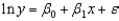
(Essay)
4.9/5 (38)
Exhibit 16-2
In a regression model involving 30 observations, the following estimated regression equation was obtained.  = 170 + 34x1 - 3x2 + 8x3 + 58x4 + 3x5
For this model, SSR = 1,740 and SST = 2,000.
-Refer to Exhibit 16-2. The degrees of freedom associated with SST are
= 170 + 34x1 - 3x2 + 8x3 + 58x4 + 3x5
For this model, SSR = 1,740 and SST = 2,000.
-Refer to Exhibit 16-2. The degrees of freedom associated with SST are
(Multiple Choice)
4.8/5 (29)
Exhibit 16-1
In a regression analysis involving 25 observations, the following estimated regression equation was developed. = 10 - 18x1 + 3x2 + 14x3
Also, the following standard errors and the sum of squares were obtained.Sb1 = 3 Sb2 = 6 Sb3 = 7
SST = 4,800 SSE = 1,296
-Refer to Exhibit 16-1. If we are interested in testing for the significance of the relationship among the variables (i.e., significance of the model) the critical value of F at = 0.05 is
(Multiple Choice)
4.8/5 (25)
A regression analysis (involving 45 observations) relating a dependent variable (y) and two independent variables resulted in the following information.  = 0.408 + 1.3387x1 + 2x2
The SSE for the above model is 49.When two other independent variables were added to the model, the following information was provided.
= 0.408 + 1.3387x1 + 2x2
The SSE for the above model is 49.When two other independent variables were added to the model, the following information was provided.  = 1.2 + 3.0x1 + 12x2 + 4.0x3 + 8x4
This latter model's SSE is 40.At a 5% significance level, test to determine if the two added independent variables contribute significantly to the model.
= 1.2 + 3.0x1 + 12x2 + 4.0x3 + 8x4
This latter model's SSE is 40.At a 5% significance level, test to determine if the two added independent variables contribute significantly to the model.
(Essay)
4.9/5 (32)
Monthly total production costs and the number of units produced at a local company over a period of 10 months are shown below.  a.Draw a scatter diagram for the above data.
b.Assume that a model in the form of
y = 0 + 1+
best describes the relationship between x and y. Estimate the parameters of this curvilinear regression equation.
a.Draw a scatter diagram for the above data.
b.Assume that a model in the form of
y = 0 + 1+
best describes the relationship between x and y. Estimate the parameters of this curvilinear regression equation.
(Essay)
4.9/5 (42)
The joint effect of two variables acting together is called
(Multiple Choice)
4.7/5 (37)
A soft drink manufacturer has developed a regression model relating sales (y in $10,000) with four independent variables. The four independent variables are price per unit (x1, in dollars), competitor's price (x2, in dollars), advertising (x3, in $1000) and type of container used (x4; 1 = Cans and 0 = Bottles). Part of the regression results are shown below. (Assume n = 25)  a.If the manufacturer uses can containers and if his price is $1.25, his advertising expenditure is $200,000, and his competitor's price is $1.50, what is your estimate of his sales? (Give your answer in dollars.)
b.Test to see if there is a significant relationship between sales and unit price. Let = 0.05.
c.Test to see if there is a significant relationship between sales and advertising. Let = 0.05.
d.Is the type of container a significant variable? Let = 0.05 = 0.05.
e.Test to see if there is a significant relationship between sales and competitor's price. Let = 0.05.
a.If the manufacturer uses can containers and if his price is $1.25, his advertising expenditure is $200,000, and his competitor's price is $1.50, what is your estimate of his sales? (Give your answer in dollars.)
b.Test to see if there is a significant relationship between sales and unit price. Let = 0.05.
c.Test to see if there is a significant relationship between sales and advertising. Let = 0.05.
d.Is the type of container a significant variable? Let = 0.05 = 0.05.
e.Test to see if there is a significant relationship between sales and competitor's price. Let = 0.05.
(Essay)
4.9/5 (35)
Exhibit 16-2
In a regression model involving 30 observations, the following estimated regression equation was obtained. = 170 + 34x1 - 3x2 + 8x3 + 58x4 + 3x5
For this model, SSR = 1,740 and SST = 2,000.
-Refer to Exhibit 16-2. The value of MSE is
(Multiple Choice)
4.8/5 (33)
The correlation in error terms that arises when the error terms at successive points in time are related is termed
(Multiple Choice)
4.8/5 (34)
Multiple regression analysis was used to study the relationship between a dependent variable, y, and three independent variables x1, x2 and, x3. The following is a partial result of the regression analysis involving 20 observations.  a.Compute the coefficient of determination.
b.Perform a t test and determine whether or not 1 is significantly different from zero ( = 0.05).
c.Perform a t test and determine whether or not 2 is significantly different from zero ( = 0.05).
d.Perform a t test and determine whether or not 3 is significantly different from zero ( = 0.05).
e.At = 0.05, perform an F test and determine whether or not the regression model is significant.
a.Compute the coefficient of determination.
b.Perform a t test and determine whether or not 1 is significantly different from zero ( = 0.05).
c.Perform a t test and determine whether or not 2 is significantly different from zero ( = 0.05).
d.Perform a t test and determine whether or not 3 is significantly different from zero ( = 0.05).
e.At = 0.05, perform an F test and determine whether or not the regression model is significant.
(Essay)
4.9/5 (44)
Exhibit 16-4
In a laboratory experiment, data were gathered on the life span (y in months) of 33 rats, units of daily protein intake (x1), and whether or not agent x2 (a proposed life extending agent) was added to the rats diet (x2 = 0 if agent x2 was not added, and x2 = 1 if agent was added.) From the results of the experiment, the following regression model was developed.  = 36 + 0.8x1 - 1.7x2
Also provided are SSR = 60 and SST = 180.
-Refer to Exhibit 16-4. From the above function, it can be said that the life expectancy of rats that were given agent x2 is
= 36 + 0.8x1 - 1.7x2
Also provided are SSR = 60 and SST = 180.
-Refer to Exhibit 16-4. From the above function, it can be said that the life expectancy of rats that were given agent x2 is
(Multiple Choice)
4.8/5 (32)
Monthly total production costs and the number of units produced at a local company over a period of 10 months are shown below.  Use Excel's Regression Tool to estimate a second-order model of the form
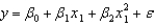
(Essay)
5.0/5 (38)
Excel's Regression tool can be used to perform the ____ procedure.
(Multiple Choice)
4.8/5 (44)
Which of the following tests is used to determine whether an additional variable makes a significant contribution to a multiple regression model?
(Multiple Choice)
4.8/5 (33)
Exhibit 16-2
In a regression model involving 30 observations, the following estimated regression equation was obtained. = 170 + 34x1 - 3x2 + 8x3 + 58x4 + 3x5
For this model, SSR = 1,740 and SST = 2,000.
-Refer to Exhibit 16-2. The computed F value for testing the significance of the above model is
(Multiple Choice)
4.9/5 (35)
The following estimated regression equation has been developed for the relationship between y, the dependent variable, and x, the independent variable. 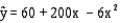 The sample size for this regression model was 23, and SSR = 600 and SSE = 400.
a.Compute the coefficient of determination.
b.Using = .05, test for a significant relationship.
The sample size for this regression model was 23, and SSR = 600 and SSE = 400.
a.Compute the coefficient of determination.
b.Using = .05, test for a significant relationship.
(Essay)
4.9/5 (34)
Exhibit 16-4
In a laboratory experiment, data were gathered on the life span (y in months) of 33 rats, units of daily protein intake (x1), and whether or not agent x2 (a proposed life extending agent) was added to the rats diet (x2 = 0 if agent x2 was not added, and x2 = 1 if agent was added.) From the results of the experiment, the following regression model was developed. = 36 + 0.8x1 - 1.7x2
Also provided are SSR = 60 and SST = 180.
-Refer to Exhibit 16-4. The life expectancy of a rat that was not given any protein and that did not take agent x2 is
(Multiple Choice)
4.8/5 (40)
Filters
- Essay(0)
- Multiple Choice(0)
- Short Answer(0)
- True False(0)
- Matching(0)