Exam 12: B: linear Regression and Correlation

Oil Quality and Price Narrative Quality of oil is measured in API gravity degrees; the higher the degrees API, the higher the quality. The table shown below was produced by an expert in the field who believes that there is a relationship between quality and price per barrel. A partial MINITAB output follows: Descriptive Statistics Covariances Degrees Price Degrees 21.281667 Price 2.026750 0.208833 Regression Analysis S = 0.1314 R-Sq = 92.46% R-Sq(adj) = 91.7% Analysis of Variance -Refer to Oil Quality and Price Narrative. Use the equation 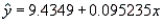to determine the predicted values of y.

Income and Education Narrative A professor of economics wants to study the relationship between income (y in $1,000s) and education (x in years). A random sample eight individuals is taken and the results are shown below. -Refer to Income and Education Narrative. Determine the least-squares regression line.

Ice Cream Sales Narrative The manager of an ice cream store is interested in examining the relationship between sales of ice cream (in litres per day) and maximum temperature of the day. The vendor records the following data for a random sample of five days in the summer, where y is number of litres of ice cream sold per day and x is maximum temperature, in degrees Celsius, recorded for the day: The following summary information was computed: -Refer to Ice Cream Sales Narrative. Find and interpret the coefficient of determination.

Amount of Trees and Beavers A scientist is studying the relationship between x = density (in number per square metre) of aspen trees around a pond and y = beaver abundance. The following statistical software output is from a regression analysis for predicting y from x. s = 0.4839 R-sq = 97.0% R-sq(adj) = 96.5% Analysis of Variance -Refer to Amount of Trees and Beavers. What are the estimated slope and estimated intercept?

Sleep Deprivation Narrative A study was conducted to determine the effects of sleep deprivation on people's ability to solve s. The amount of sleep deprivation varied with 8, 12, 16, 20, and 24 hours without sleep. A total of ten subjects participated in the study, two at each sleep deprivation level. After his or her specified sleep deprivation period, each subject was administered a set of simple addition s, and the number of errors was recorded. These results were obtained: -Refer to Sleep Deprivation Narrative. Would you expect the relationship between y and x to be linear if x varied over a wider range (say, x = 4 to x = 48)?

Income and Height Narrative Do tall men earn more than short ones? An economist collected the data shown below for 25 men, where the annual income (y) in thousands of dollars and the height of the income earner (x) in cm. -Refer to Income and Height Narrative. Do the data present sufficient evidence to indicate that annual income and height of income earner are linearly related? Use the F test at the 5% level of significance.

Blacktop Let x be the area (in square metres) to be covered with blacktop, and let y be the time (in minutes) it takes a construction crew to completely cover the area. The simple linear regression model relates x and y where the least-squares estimates of the regression parameters are b = 0.207 and a = 81.6. -Refer to Blacktop statement. What is the least-squares best-fitting regression line?

TV Game Show Revenues Narrative An ardent fan of television game shows has observed that, in general, the more educated the contestant, the less money he or she wins. To test her belief, she gathers data about the last eight winners of her favourite game show. She records their winnings in dollars and the number of years of education. The results are as follows. -Refer to TV Game Show Revenues Narrative. Estimate with 95% confidence the average winnings of all contestants who have ten years of education.

Microwave Sales Narrative A microwave oven manufacturer has collected the data shown below on number of units sold (y) in the thousands of dollars and the number of ads (x) placed during the month. -Refer to Microwave Sales Narrative. Calculate the quantities SSE and MSE.

Wind Velocity and Windmills Narrative A scientist is studying the relationship between wind velocity (x in km/h) and DC output of a windmill (y). The following MINITAB output is from a regression analysis for predicting y from x. s = 0.2435 R-sq = 88.3% R-sq(adj) = 87.3% Analysis of Variance -Refer to Wind Velocity and Windmills Narrative. . Identify and interpret the coefficient of determination.

Oil Quality and Price Narrative Quality of oil is measured in API gravity degrees; the higher the degrees API, the higher the quality. The table shown below was produced by an expert in the field who believes that there is a relationship between quality and price per barrel. A partial MINITAB output follows: Descriptive Statistics Covariances Degrees Price Degrees 21.281667 Price 2.026750 0.208833 Regression Analysis S = 0.1314 R-Sq = 92.46% R-Sq(adj) = 91.7% Analysis of Variance -Refer to Oil Quality and Price Narrative. Does it appear that the errors are normally distributed? Explain.

Young Aspen Trees and Growth Narrative Let x be the number of leaves on a young aspen tree and let y be the growth of the tree (in mm). The data are as follows. -Refer to Young Aspen Trees and Growth Narrative. Find and interpret the coefficient of determination.

Sunshine and Skin Cancer Narrative A medical statistician wanted to examine the relationship between the amount of sunshine (x) in hours, and incidence of skin cancer (y). As an experiment, he found the number of skin cancers detected per 100,000 of population and the average daily sunshine in eight counties around the country. These data are shown below: -Refer to Sunshine and Skin Cancer Narrative. What does the value of the slope of the regression line tell you?

TV Game Show Revenues Narrative An ardent fan of television game shows has observed that, in general, the more educated the contestant, the less money he or she wins. To test her belief, she gathers data about the last eight winners of her favourite game show. She records their winnings in dollars and the number of years of education. The results are as follows. -Refer to TV Game Show Revenues Narrative. Predict with 95% confidence the winnings of a contestant who has ten years of education.

Forest Age and Tree Diameter Narrative A scientist is studying the relationship between the age of a forest, x, in years and the average diameter of the trees, y, in cm. One study reported the following data. -Refer to Forest Age and Tree Diameter. Develop a 95% prediction interval of y when x = 83.

Income and Education Narrative A professor of economics wants to study the relationship between income (y in $1,000s) and education (x in years). A random sample eight individuals is taken and the results are shown below. -Refer to Income and Education Narrative. Which interval in the previous two questions is narrower: the confidence interval estimate of the expected value of y or the prediction interval for the same given value of x (ten years) and same confidence level? Why?

Income and Education Narrative A professor of economics wants to study the relationship between income (y in $1,000s) and education (x in years). A random sample eight individuals is taken and the results are shown below. -Refer to Income and Education Narrative. Conduct a test of the population slope to determine at the 5% significance level whether a linear relationship exists between years of education and income.

Income and Height Narrative Do tall men earn more than short ones? An economist collected the data shown below for 25 men, where the annual income (y) in thousands of dollars and the height of the income earner (x) in cm. -Refer to Income and Height Narrative. Predict the annual income for a 6-foot-tall man.

Circumference and Age Narrative Evidence supports using a simple linear regression model to estimate the circumference of a pine tree based on its age. Let x be the age of the pine tree (measured in years) and y be the circumference (measured in cm). A random sample of 11 mature pine trees was selected and the following data recorded: The following output was generated using statistical software: 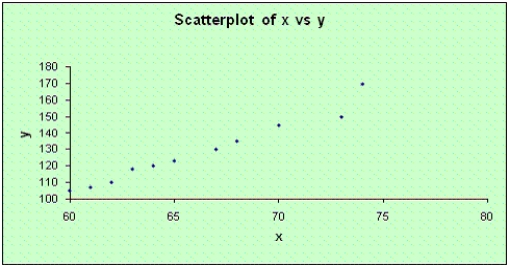Regression Analysis The regression equation is y = -148 + 4.18x S = 4.025 R-Sq = 96.4% R-Sq(adj) = 96.0% Analysis of Variance Table Unusual Observations R denotes an observation with a large standardized residual -Six points have these coordinates: The normal probability plot and the residuals versus fitted values plots generated by statistical software are shown below. Does it appear that any regression assumptions have been violated? Explain.

Vending Machines Narrative Let x be the number of vending machines and let y be the time (in hours) it takes to stock them. The data are as follows. -Refer to Vending Machines Narrative. What is the equation of the estimated regression line?