Exam 12: B: linear Regression and Correlation

Young Aspen Trees and Growth Narrative Let x be the number of leaves on a young aspen tree and let y be the growth of the tree (in mm). The data are as follows. -Refer to Young Aspen Trees and Growth Narrative. What is the average change in growth with the increase of one leaf?

Advertising and Money Spent Narrative A marketing analyst is studying the relationship between x = money spent on television advertising and y = increase in sales. One study reported the following data (in dollars) for a particular company. -Refer to Advertising and Money Spent Narrative. Does a linear relationship exist between x and y? Test using = 0.05.

Sunshine and Skin Cancer Narrative A medical statistician wanted to examine the relationship between the amount of sunshine (x) in hours, and incidence of skin cancer (y). As an experiment, he found the number of skin cancers detected per 100,000 of population and the average daily sunshine in eight counties around the country. These data are shown below: -Refer to Sunshine and Skin Cancer Narrative. Determine the least-squares regression line.

Oil Quality and Price Narrative Quality of oil is measured in API gravity degrees; the higher the degrees API, the higher the quality. The table shown below was produced by an expert in the field who believes that there is a relationship between quality and price per barrel. A partial MINITAB output follows: Descriptive Statistics Covariances Degrees Price Degrees 21.281667 Price 2.026750 0.208833 Regression Analysis S = 0.1314 R-Sq = 92.46% R-Sq(adj) = 91.7% Analysis of Variance -Refer to Oil Quality and Price Narrative. Does it appear that random variables is a ? Explain.

Antibiotic Potency Narrative An experiment was conducted to observe the effect of an increase in temperature on the potency of an antibiotic. Three 25 gram portions of the antibiotic were stored for equal lengths of time at each of these temperatures: C, C, C, and C. The potency readings observed at each temperature of the experimental period are listed here: -Refer to Antibiotic Potency Narrative. Suppose that a batch of the antibiotic was stored at C for the same length of time as the experimental period. Predict the potency of the batch at the end of the storage period. Use a 95% prediction interval.

Willie Nelson Concert Narrative At a recent Willie Nelson concert, a survey was conducted that asked a random sample of 20 people their age and how many concerts they have attended since the first of the year. The following data were collected: An Excel output follows: 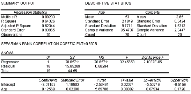-Refer to Willie Nelson Concert Narrative. Use the regression 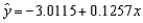to determine the predicted values of y.

Blacktop Let x be the area (in square metres) to be covered with blacktop, and let y be the time (in minutes) it takes a construction crew to completely cover the area. The simple linear regression model relates x and y where the least-squares estimates of the regression parameters are b = 0.207 and a = 81.6. -Refer to Blacktop statement. What is the estimated amount of time it takes to apply 2400 square metres of blacktop?

Salary and Years Narrative A company manager is interested in the relationship between x = number of years that an employee has been with the company and y = the employee's annual salary (in thousands of dollars). The following statistical software output is from a regression analysis for predicting y from x for n = 15 data points. s = 0.8081 R-sq = 97.9% R-sq(adj) = 97.8% -Refer to Salary and Years Narrative. Interpret the estimated slope and y-intercept for this .

Antibiotic Potency Narrative An experiment was conducted to observe the effect of an increase in temperature on the potency of an antibiotic. Three 25 gram portions of the antibiotic were stored for equal lengths of time at each of these temperatures: C, C, C, and C. The potency readings observed at each temperature of the experimental period are listed here: -Refer to Antibiotic Potency Narrative. Use the computing formulas to find the least-squares line appropriate for these data.

Willie Nelson Concert Narrative At a recent Willie Nelson concert, a survey was conducted that asked a random sample of 20 people their age and how many concerts they have attended since the first of the year. The following data were collected: An Excel output follows: -Refer to Willie Nelson Concert Narrative. Use the predicted values and the actual values of y to calculate the residuals.

Amount of Trees and Beavers A scientist is studying the relationship between x = density (in number per square metre) of aspen trees around a pond and y = beaver abundance. The following statistical software output is from a regression analysis for predicting y from x. s = 0.4839 R-sq = 97.0% R-sq(adj) = 96.5% Analysis of Variance -Refer to Amount of Trees and Beavers. What is the value of the coefficient of determination?

Correlation between Shoreline Erosion and Rainfall A scientist is studying the relationship between x = centimetres of annual rainfall and y = centimetres of shoreline erosion. One study reported the following data. Use the following statistical software output to answer the questions below. s = 0.2416 R-sq = 98.8% R-sq(adj) = 98.6% Analysis of Variance -Refer to Correlation Between Shoreline Erosion and Rainfall. Identify and interpret the coefficient of determination.

Sales and Experience Narrative The general manager of a chain of furniture stores believes that experience is the most important factor in determining the level of success of a salesperson. To examine this belief, she records last month's sales (in $1000s) and the years of experience of ten randomly selected salespeople. These data are listed below. -Refer to Sales and Experience Narrative. Which interval in the previous two questions is narrower: the confidence interval estimate of the expected value of y or the prediction interval for the same given value of x (ten years) and same confidence level? Why?

Sales and Experience Narrative The general manager of a chain of furniture stores believes that experience is the most important factor in determining the level of success of a salesperson. To examine this belief, she records last month's sales (in $1000s) and the years of experience of ten randomly selected salespeople. These data are listed below. -Refer to Sales and Experience Narrative. Calculate the Pearson correlation coefficient. What sign does it have? Why?

Special Programs Narrative A social skills training program was implemented with seven students with disabilities in a study to determine whether the program caused improvement in pre/post measures and behaviour ratings. For one such test, the pre- and posttest scores for the seven students are given in the table. -Refer to Special Programs Narrative. What type of correlation, if any, do you expect to see between the pre- and posttest scores? Plot the data. Does the correlation appear to be positive or negative?

Income and Height Narrative Do tall men earn more than short ones? An economist collected the data shown below for 25 men, where the annual income (y) in thousands of dollars and the height of the income earner (x) in cm. -Refer to Income and Height Narrative. Construct the scatterplot and plot the fitted line on the scatterplot. Does the assumption of a linear relationship appear to be reasonable?

SAT Scores and GPA Narrative A university admissions committee was interested in examining the relationship between a student's score on the Scholastic Aptitude Test, x, and the student's grade point average, y, at the end of the student's first year of university. The committee selected a random sample of 25 students and recorded the SAT score and GPA at the end of the first year of university for each student. Use the following output that was generated using statistical software to answer the questions below: Regression Analysis The regression equation is GPA = -1.09 + 0.00349 SAT S = 0.1463 R-Sq = 91.8% R-Sq(adj) = 91.5% Analysis of Variance Correlations (Pearson) Correlation of SAT and GPA = 0.958 -Refer to SAT Scores and GPA Narrative. Determine the correlation between a student's SAT score and GPA at the end of the freshman year. Interpret the value.

Amount of Trees and Beavers A scientist is studying the relationship between x = density (in number per square metre) of aspen trees around a pond and y = beaver abundance. The following statistical software output is from a regression analysis for predicting y from x. s = 0.4839 R-sq = 97.0% R-sq(adj) = 96.5% Analysis of Variance -Refer to Amount of Trees and Beavers. Interpret the estimated slope and intercept for this .

Oil Quality and Price Narrative Quality of oil is measured in API gravity degrees; the higher the degrees API, the higher the quality. The table shown below was produced by an expert in the field who believes that there is a relationship between quality and price per barrel. A partial MINITAB output follows: Descriptive Statistics Covariances Degrees Price Degrees 21.281667 Price 2.026750 0.208833 Regression Analysis S = 0.1314 R-Sq = 92.46% R-Sq(adj) = 91.7% Analysis of Variance -Refer to Oil Quality and Price Narrative. Draw a histogram of the residuals.

Antibiotic Potency Narrative An experiment was conducted to observe the effect of an increase in temperature on the potency of an antibiotic. Three 25 gram portions of the antibiotic were stored for equal lengths of time at each of these temperatures: C, C, C, and C. The potency readings observed at each temperature of the experimental period are listed here: -Refer to Antibiotic Potency Narrative. Estimate the mean potency corresponding to a temperature of C. Use a 95% confidence interval.