Exam 18: Simple Linear Regression and Correlation

Given that SSE = 84 and SSR = 358.12, the coefficient of correlation (also called the Pearson coefficient of correlation) must be 0.90.

Which of the following statements best describes correlation analysis in a simple linear regression?

A financier whose specialty is investing in movie productions has observed that, in general, movies with 'big-name' stars seem to generate more revenue than those movies whose stars are less well known. To examine his belief, he records the gross revenue and the payment (in $ million) given to the two highest-paid performers in the movie for 10 recently released movies. Movie Cost of two highest- paid performers (\ ) Gross revenue (\ ) 1 5.3 48 2 7.2 65 3 1.3 18 4 1.8 20 5 3.5 31 6 2.6 26 7 8.0 73 8 2.4 23 9 4.5 39 10 6.7 58 Use the regression equation to determine the predicted values of y.

A medical statistician wanted to examine the relationship between the amount of sunshine (x) and incidence of skin cancer (y). As an experiment he found the number of skin cancers detected per 100 000 of population and the average daily sunshine in eight country towns around NSW. These data are shown below. Average daily sunshine (hours) 5 7 6 7 8 6 4 3 Skin cancer per 100000 7 11 9 12 15 10 7 5 Calculate the standard error of estimate, and describe what this statistic tells you about the regression line.

Plot the residuals against the predicted values of y. Does the variance appear to be constant?

An outlier is an observation that is unusually small or unusually large.

An ardent fan of television game shows has observed that, in general, the more educated the contestant, the less money he or she wins. To test her belief, she gathers data about the last eight winners of her favourite game show. She records their winnings in dollars and their years of education. The results are as follows. Contestant Years of education Winnings 1 11 750 2 15 400 3 12 600 4 16 350 5 11 800 6 16 300 7 13 650 8 14 400 Conduct a test of the population slope to determine at the 5% significance level whether a linear relationship exists between TV game show contestants' years of education and their winnings.

A professor of economics wants to study the relationship between income y (in $1000s) and education x (in years). A random sample of eight individuals is taken and the results are shown below. Education 16 11 15 8 12 10 13 14 Income 58 40 55 35 43 41 52 49 Identify possible outliers.

Plot the residuals against the predicted values . Does the variance appear to be constant?

The editor of a major academic book publisher claims that a large part of the cost of books is the cost of paper. This implies that larger books will cost more money. As an experiment to analyse the claim, a university student visits the bookstore and records the number of pages and the selling price of 12 randomly selected books. These data are listed below. $\begin{array} { | c | c | c | } \hline \text { Book } & \text { Number of pages } & \text { Selling price (\$) } \\\hline 1 & 844 & 55 \\\hline 2 & 727 & 50 \\\hline 3 & 360 & 35 \\\hline 4 & 915 & 60 \\\hline 5 & 295 & 30 \\\hline 6 & 706 & 50 \\\hline 7 & 410 & 40 \\\hline 8 & 905 & 53 \\\hline 9 & 1058 & 65 \\\hline 10 & 865 & 54 \\\hline 11 & 677 & 42 \\\hline 12 & 912 & 58 \\\hline\end{array}$ Can we infer at the 5% significance level that the editor is correct?

In the first-order linear regression model, the population parameters of the y-intercept and the slope are estimated by:

A professor of economics wants to study the relationship between income y (in $1000s) and education x (in years). A random sample of eight individuals is taken and the results are shown below. Education 16 11 15 8 12 10 13 14 Income 58 40 55 35 43 41 52 49 Compute the standardised residuals.

A regression analysis between sales (in $1000) and advertising (in $100) yielded the least squares line y-hat = 77 +8x. This implies that if advertising is $600, then the predicted amount of sales (in dollars) is $4877.

Predict weekly sales in the fast food restaurant if 5 vouchers are printed in the local newspaper, given, Estimated Sales = 11.5676 + 0.4618.Vouchers Is this a good estimate?

The editor of a major academic book publisher claims that a large part of the cost of books is the cost of paper. This implies that larger books will cost more money. As an experiment to analyse the claim, a university student visits the bookstore and records the number of pages and the selling price of 12 randomly selected books. These data are listed below. $\begin{array} { | c | c | c | } \hline \text { Book } & \text { Number of pages } & \text { Selling price (\$) } \\\hline 1 & 844 & 55 \\\hline 2 & 727 & 50 \\\hline 3 & 360 & 35 \\\hline 4 & 915 & 60 \\\hline 5 & 295 & 30 \\\hline 6 & 706 & 50 \\\hline 7 & 410 & 40 \\\hline 8 & 905 & 53 \\\hline 9 & 1058 & 65 \\\hline 10 & 865 & 54 \\\hline 11 & 677 & 42 \\\hline 12 & 912 & 58 \\\hline\end{array}$ Determine the coefficient of determination, and discuss what its value tells you.

In simple linear regression, the divisor of the standard error of estimate, $S _ { \varepsilon }$ , is n - 1.

Plot the residuals against the predicted values of y. Does the variance appear to be constant?

Consider the following data values of variables x and y. x 3 5 7 9 11 14 y 7 10 17 20 27 35 Calculate the coefficient of determination, and describe what this statistic tells you about the relationship between the two variables.

At a recent music concert, a survey was conducted that asked a random sample of 20 people their age and how many concerts they have attended since the beginning of the year. The following data were collected. Age 62 57 40 49 67 54 43 65 54 41 Number of concerts 6 5 4 3 5 5 2 6 3 1 Age 44 48 55 60 59 63 69 40 38 52 Number of Concerts 3 2 4 5 4 5 4 2 1 3 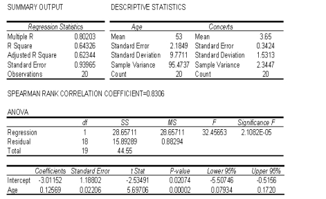a. Draw a scatter diagram of the data to determine whether a linear model appears to be appropriate to describe the relationship between the age and number of concerts attended by the respondents. b. Determine the least squares regression line. c. Plot the least squares regression line. d. Interpret the value of the slope of the regression line.

A statistician investigating the relationship between the amount of precipitation (in inches) and the number of car accidents gathered data for 10 randomly selected days. The results are presented below. Day Precipitation Number of accidents 1 0.05 5 2 0.12 6 3 0.05 2 4 0.08 4 5 0.10 8 6 0.35 14 7 0.15 7 8 0.30 13 9 0.10 7 10 0.20 10 Calculate the standard error of estimate, and describe what this statistic tells you about the regression line.