Exam 18: Simple Linear Regression and Correlation
Exam 1: What Is Statistics14 Questions
Exam 2: Types of Data, Data Collection and Sampling16 Questions
Exam 3: Graphical Descriptive Methods Nominal Data19 Questions
Exam 4: Graphical Descriptive Techniques Numerical Data64 Questions
Exam 5: Numerical Descriptive Measures147 Questions
Exam 6: Probability106 Questions
Exam 7: Random Variables and Discrete Probability Distributions55 Questions
Exam 8: Continuous Probability Distributions117 Questions
Exam 9: Statistical Inference: Introduction8 Questions
Exam 10: Sampling Distributions65 Questions
Exam 11: Estimation: Describing a Single Population127 Questions
Exam 12: Estimation: Comparing Two Populations22 Questions
Exam 13: Hypothesis Testing: Describing a Single Population129 Questions
Exam 14: Hypothesis Testing: Comparing Two Populations78 Questions
Exam 15: Inference About Population Variances49 Questions
Exam 16: Analysis of Variance115 Questions
Exam 17: Additional Tests for Nominal Data: Chi-Squared Tests110 Questions
Exam 18: Simple Linear Regression and Correlation213 Questions
Exam 19: Multiple Regression121 Questions
Exam 20: Model Building92 Questions
Exam 21: Nonparametric Techniques126 Questions
Exam 22: Statistical Inference: Conclusion103 Questions
Exam 23: Time-Series Analysis and Forecasting145 Questions
Exam 24: Index Numbers25 Questions
Exam 25: Decision Analysis51 Questions
Select questions type
An ardent fan of television game shows has observed that, in general, the more educated the contestant, the less money he or she wins. To test her belief, she gathers data about the last eight winners of her favourite game show. She records their winnings in dollars and their years of education. The results are as follows. Contestant Years of education Winnings 1 11 750 2 15 400 3 12 600 4 16 350 5 11 800 6 16 300 7 13 650 8 14 400 Use the regression equation to determine the predicted values of y.
(Essay)
4.8/5  (39)
(39)
A statistician investigating the relationship between the amount of precipitation (in inches) and the number of car accidents gathered data for 10 randomly selected days. The results are presented below. Day Precipitation Number of accidents 1 0.05 5 2 0.12 6 3 0.05 2 4 0.08 4 5 0.10 8 6 0.35 14 7 0.15 7 8 0.30 13 9 0.10 7 10 0.20 10 Predict with 95% confidence the number of accidents that occur when there is 0.40 inches of rain.
(Essay)
4.9/5 (33)
When the actual values y of a dependent variable and the corresponding predicted values  are the same, the standard error of estimate, , will be 0.0.
(True/False)
4.9/5 (24)
A television rating wants to determine whether married couples tend to agree about the quality of the television shows they watch. Ten couples are asked to rate a particular comedy series on a 7-point scale where 1 = terrible and 7 = excellent. The results are shown below. Husband's rating 3 6 6 5 4 5 7 4 5 5 Wife's rating 5 5 4 5 4 4 6 3 4 5 Do these data provide sufficient evidence at the 5% significance level to conclude that the husband's and the wife's ratings are positively related?
(Essay)
4.7/5 (40)
In regression analysis, if the coefficient of correlation is -1.0, then:
(Multiple Choice)
4.8/5 (31)
The least squares method requires that the variance of the error variable is a constant no matter what the value of x is. When this requirement is violated, the condition is called:
(Multiple Choice)
4.8/5 (41)
The following sums of squares are produced:  (yi-(y-bar))2 = 250, 11ef1ab2_4bf1_c05d_a741_c73dacf30ae9_TB5762_11(yi-(yi-hat))2 = 100, 11ef1ab2_4bf1_c05d_a741_c73dacf30ae9_TB5762_11((yi-hat)-(y-bar))2 = 150
The percentage of the variation in y that is explained by the variation in x is:
(yi-(y-bar))2 = 250, 11ef1ab2_4bf1_c05d_a741_c73dacf30ae9_TB5762_11(yi-(yi-hat))2 = 100, 11ef1ab2_4bf1_c05d_a741_c73dacf30ae9_TB5762_11((yi-hat)-(y-bar))2 = 150
The percentage of the variation in y that is explained by the variation in x is:
(Multiple Choice)
4.9/5 (35)
Correlation analysis is used to determine the strength of a non-linear relationship between an independent variable x and a dependent variable y.
(True/False)
4.9/5 (35)
A medical statistician wanted to examine the relationship between the amount of sunshine (x) and incidence of skin cancer (y). As an experiment he found the number of skin cancers detected per 100 000 of population and the average daily sunshine in eight country towns around NSW. These data are shown below. Average daily sunshine (hours) 5 7 6 7 8 6 4 3 Skin cancer per 100000 7 11 9 12 15 10 7 5 Draw a scatter diagram of the data and plot the least squares regression line on it.
(Essay)
4.8/5 (31)
A regression line using 25 observations produced SSR = 118.68 and SSE = 56.32. The standard error of estimate was:
(Multiple Choice)
4.8/5 (43)
The manager of a fast food restaurant wants to determine how sales in a given week are related to the number of discount vouchers (#) printed in the local newspaper during the week. The number of vouchers and sales ($000s) from 10 randomly selected weeks is given below with the predicted sales.
Calculate the residuals. observation Sales predicted Sales 1 12.8 13.4147 2 15.4 14.8000 3 13.9 13.8765 4 11.2 12.9529 5 18.7 20.3412 6 17.9 16.1853 7 16.8 15.2618 8 15.9 14.3382 9 11.5 12.9529 10 13.9 13.8765
(Essay)
4.8/5 (28)
We standardise residuals in the same way that we standardise all variables, by subtracting the mean and dividing by the variance.
(True/False)
4.8/5 (41)
In developing a 95% confidence interval for the expected value of y from a simple linear regression problem involving a sample of size 10, the appropriate table value would be 2.306.
(True/False)
4.8/5 (29)
A statistician investigating the relationship between the amount of precipitation (in inches) and the number of car accidents gathered data for 10 randomly selected days. The results are presented below. Day Precipitation Number of accidents 1 0.05 5 2 0.12 6 3 0.05 2 4 0.08 4 5 0.10 8 6 0.35 14 7 0.15 7 8 0.30 13 9 0.10 7 10 0.20 10 Find the least squares regression line.
(Essay)
4.8/5 (37)
A statistician investigating the relationship between the amount of precipitation (in inches) and the number of car accidents gathered data for 10 randomly selected days. The results are presented below. Day Precipitation Number of accidents 1 0.05 5 2 0.12 6 3 0.05 2 4 0.08 4 5 0.10 8 6 0.35 14 7 0.15 7 8 0.30 13 9 0.10 7 10 0.20 10 Estimate with 95% confidence the mean daily number of accidents when the daily precipitation is 0.25 inches.
(Essay)
4.9/5 (36)
The symbol for the population coefficient of correlation is:
(Multiple Choice)
4.7/5 (30)
In a regression problem, if all the values of the independent variable are equal, then the coefficient of determination must be:
(Multiple Choice)
4.9/5 (33)
A regression analysis between y, sales (in $1000) and x, advertising (in $) yielded the least squares line
= 60 + 5x. We can interpret the slope by saying that we estimate for each extra $1 spent on advertising that sales will increase by $5 000, on average.
(True/False)
4.9/5 (34)
The manager of a fast food restaurant wants to determine how sales in a given week are related to the number of discount vouchers (#) printed in the local newspaper during the week. The number of vouchers and sales ($000s) from 10 randomly selected weeks is given below with Excel regression output. Number of vo uchers Sales 4 12.8 7 15.4 5 13.9 3 11.2 19 18.7 10 17.9 8 16.8 6 15.9 3 11.5 5 13.9 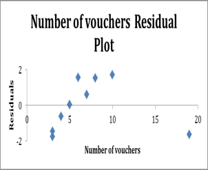 Identify possible outliers.
(Essay)
4.8/5 (27)
Filters
- Essay(0)
- Multiple Choice(0)
- Short Answer(0)
- True False(0)
- Matching(0)