Exam 12: Multiple Regression and Model Building

A study of the top MBA programs attempted to predict $y =$ the average starting salary (in $\$ 1000$ 's) of graduates of the program based on $x =$ the amount of tuition (in $\$ 1000$ 's) charged by the program. After first considering a simple linear model, it was decided that a quadratic model should be proposed. Which of the following models proposes a 2nd-order quadratic relationship between $x$ and $y$ ?

A fast food chain test marketing a new sandwich chose 18 of its stores in one major metropolitan area. Nine of the stores were in malls and nine were free standing. The sandwich was offered at three different introductory prices. The table shows the number of new sandwiches sold at each location for each location type and price combination. Number of New Sandwiches Sold 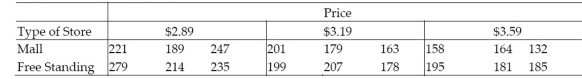a. Write a model for the mean number of sandwiches sold, $E ( y )$ , assuming that the relationship between $E ( y )$ and price, $x _ { 1 }$ , is first-order. b. Fit the model to the data. c. Write the prediction equations for mall and free-standing stores. d. Do the data provide sufficient evidence that the change in number of sandwiches sold with respect to price is different for mall and free-standing stores? Use $\alpha = .01$ .

A study of the top MBA programs attempted to predict the average starting salary (in $1000ʹs)of graduates of the program based on the amount of tuition (in $1000ʹs)charged by the program and The average GMAT score of the programʹs students. The results of a regression analysis based on a Sample of 75 MBA programs is shown below: Least Squares Linear Regression of Salary Predictor Variables Coefficient Std Error T P VIF Constant -203.402 51.6573 -3.94 0.0002 0.0 Gmat 0.39412 0.09039 4.36 0.0000 2.0 Tuition 0.92012 0.17875 5.15 0.0000 2.0 R-Squared 0.6857 Resid. Mean Square (MSE) 427.511 Adjusted R-Squared 0.6769 Standard Deviation 20.6763 Interpret the coefficient for the tuition variable shown on the printout.

It is safe to conduct t-tests on the individual β parameters in a first-order linear model in order to determine which independent variables are useful for predicting y and which are not.

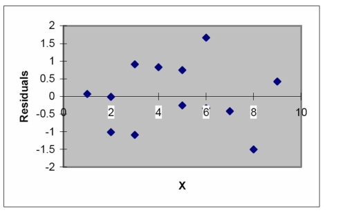
It is desired to build a regression model to predict $y =$ the sales price of a single family home, based on the $x _ { 1 } =$ size of the house and $x _ { 2 } =$ the neighborhood the home is located in. The goal is to compare the prices of homes that are located in two different neighborhoods. The following model is proposed: $\mathrm { E } ( \mathrm { y } ) = \beta _ { 0 } + \beta _ { 1 } \mathrm { x } _ { 1 } + \beta _ { 2 } \mathrm { x } _ { 2 }$ A regression model was fit and the following residual plot was observed. Which of the following assumptions appears violated based on this plot?

Consider the model $y = \beta _ { 0 } + \beta _ { 1 } x _ { 1 } + \beta _ { 2 } x _ { 2 } + \beta _ { 3 } x _ { 3 } + \varepsilon$ where $x _ { 1 }$ is a quantitative variable and $x _ { 2 }$ and $x _ { 3 }$ are dummy variables describing a qualitative variable at three levels using the coding scheme $x _ { 2 } = \left\{ \begin{array} { l l } 1 & \text { if level } 2 \\ 0 & \text { otherwise } \end{array} \quad x _ { 3 } = \left\{ \begin{array} { l l } 1 & \text { if level } 3 \\ 0 & \text { otherwise } \end{array} \right. \right.$ The resulting least squares prediction equation is $\hat { y } = 36.7 + 1.3 x _ { 1 } + 5.4 x _ { 2 } + 3.2 x _ { 3 }$ . What is the least squares regression equation associated with level 2?

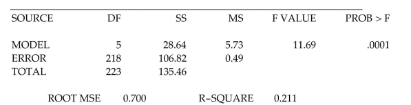
As part of a study at a large university, data were collected on n = 224 freshmen computer science (CS)majors in a particular year. The researchers were interested in modeling y, a studentʹs grade point average (GPA)after three semesters, as a function of the following independent variables (recorded at the time the students enrolled in the university): $x _ { 1 } =$ average high school grade in mathematics (HSM) $x _ { 2 } =$ average high school grade in science (HSS) $x _ { 3 } =$ average high school grade in English (HSE) $x _ { 4 } =$ SAT mathematics score (SATM) $x _ { 5 } =$ SAT verbal score (SATV) 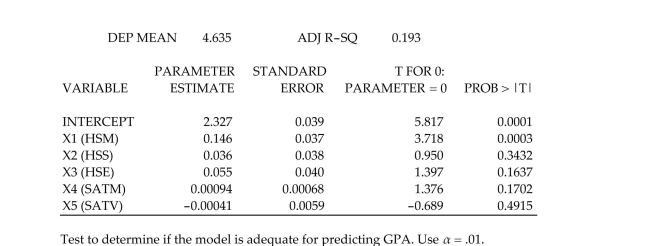A first-order model was fit to the data with the following results:

A first-order model does not contain any higher-order terms.

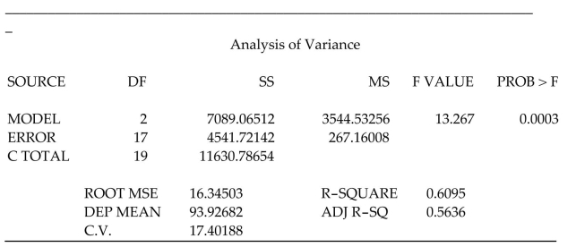
The concessions manager at a beachside park recorded the high temperature, the number of people at the park, and the number of bottles of water sold for each of 12 consecutive Saturdays. The data are shown below. Bottles Sold Temperature People 341 73 1625 425 79 2100 457 80 2125 485 80 2800 469 81 2550 395 82 1975 511 83 2675 549 83 2800 543 85 2850 537 88 2775 621 89 2800 897 91 3100 a. Fit the model $E ( y ) = \beta _ { 0 } + \beta _ { 1 } x _ { 1 } + \beta _ { 2 } x _ { 2 } + \beta _ { 3 } x _ { 1 } x _ { 2 }$ to the data, letting $y$ represent the number of bottles of water sold, $x _ { 1 }$ the temperature, and $x _ { 2 }$ the number of people at the park. b. Identify at least two indicators of multicollinearity in the model. c. Comment on the usefulness of the model to predict the number of bottles of water sold on a Saturday when the high temperature is $103 ^ { \circ } \mathrm { F }$ and there are 3500 people at the park.

Which residual plot would you examine to determine whether the assumption of constant error variance is satisfied for a model with two independent variables $x _ { 1 }$ and $x _ { 2 }$ ?

The model $E ( y ) = \beta _ { 0 } + \beta _ { 1 } x _ { 1 } + \beta _ { 2 } x _ { 2 } + \beta _ { 3 } x _ { 3 }$ was used to relate $E ( y )$ to a single qualitative variable. How many levels does the qualitative variable have?

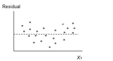
The model $E ( y ) = \beta _ { 0 } + \beta _ { 1 } x$ was fit to a set of data, and the following plot of residuals against $x$ values was obtained. Interpret the residual plot.

A study of the top MBA programs attempted to predict the average starting salary (in $1000ʹs)of graduates of the program based on the amount of tuition (in $1000ʹs)charged by the program and The average GMAT score of the programʹs students. The results of a regression analysis based on a Sample of 75 MBA programs is shown below: Least Squares Linear Regression of Salary Predictor Cases Included 75 Missing Cases 0 One of the $t$ -test test statistics is shown on the printout to be the value $t = 6.03$ . Interpret this value.

In any production process in which one or more workers are engaged in a variety of tasks, the total time spent in production varies as a function of the size of the workpool and the level of output of the various activities. In a large metropolitan department store, it is believed that the number of man-hours worked $( y )$ per day by the clerical staff depends on the number of pieces of mail processed per day $\left( x _ { 1 } \right)$ and the number of checks cashed per day $\left( x _ { 2 } \right)$ . Data collected for $n = 20$ working days were used to fit the model: $E ( y ) = \beta _ { 0 } + \beta _ { 1 } x _ { 1 } + \beta _ { 2 } x _ { 2 }$ A partial printout for the analysis follows: 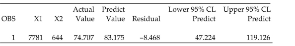Interpret the $95 \%$ prediction interval for $y$ shown on the printout.

In stepwise regression, the probability of making one or more Type I or Type II errors is quite small.

In any production process in which one or more workers are engaged in a variety of tasks, the total time spent in production varies as a function of the size of the workpool and the level of output of the various activities. In a large metropolitan department store, it is believed that the number of man-hours worked $( y )$ per day by the clerical staff depends on the number of pieces of mail processed per day $\left( x _ { 1 } \right)$ and the number of checks cashed per day $\left( x _ { 2 } \right)$ . Data collected for $n = 20$ working days were used to fit the model: $E ( y ) = \beta _ { 0 } + \beta _ { 1 } x _ { 1 } + \beta _ { 2 } x _ { 2 }$ A partial printout for the analysis follows: Test to determine if the model is adequate for predicting the number of man-hours worked. Use $\alpha = .025$ .

In Hawaii, proceedings are under way to enable private citizens to own the property that their homes are built on. In prior years, only estates were permitted to own land, and homeowners leased the land from the estate. In order to comply with the new law, a large Hawaiian estate wants to use regression analysis to estimate the fair market value of the land. The following variables are proposed: y= Sale price of property (\ thousands) =1 if property near Cove, 0 if not Write a regression model relating the sale price of a property to the qualitative variable $x$ . Interpret all the $\beta \mathrm { s }$ in the model.

Consider the partial printout below. Coefficients Standard Error t Stat P-value Lower 95\% Upper 95\% Intercept -63.14873931 25.09115112 -2.516773304 0.045484943 -124.5446192 -1.752859365 X1 14.72507864 8.113581741 1.814867849 0.119466699 -5.128155197 34.57831248 X2 12.48784546 4.686063743 2.664890224 0.037279879 1.021452165 23.95423875 X1X2 -1.886935135 1.344999834 -1.402925924 0.210210141 -5.178033575 1.404163305 Is there evidence (at \alpha=.05 ) that and interact? Explain.

One of three surfaces is produced by a complete second-order model with two quantitative independent variables: a paraboloid that opens upward, a paraboloid that opens downward, or a saddle-shaped surface.

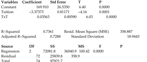
A certain type of rare gem serves as a status symbol for many of its owners. In theory, for low prices, the demand decreases as the price of the gem increases. However, experts hypothesize that When the gem is valued at very high prices, the demand increases with price due to the status the Owners believe they gain by obtaining the gem. Thus, the model proposed to best explain the Demand for the gem by its price is the quadratic model $E ( y ) = \beta _ { 0 } + \beta _ { 1 } x + \beta _ { 2 } x ^ { 2 }$ where y = Demand (in thousands)and x = Retail price per carat (dollars). This model was fit to data collected for a sample of 12 rare gems. If the experts are correct in their assumptions about the relationship between price and demand, which of the following should be true?