Exam 12: Multiple Regression and Model Building

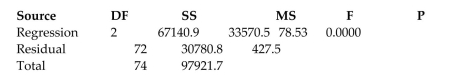
A study of the top MBA programs attempted to predict the average starting salary (in $1000ʹs)of graduates of the program based on the amount of tuition (in $1000ʹs)charged by the program and The average GMAT score of the programʹs students. The results of a regression analysis based on a Sample of 75 MBA programs is shown below: Least Squares Linear Regression of Salary 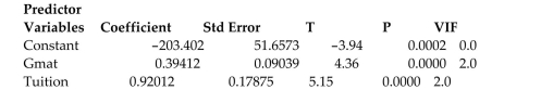R-Squared 0.6857 Resid. Mean Square (MSE) 427.511 Adjusted R-Squared 0.6769 Standard Deviation 20.6763 Interpret the coefficient of determination value shown in the printout.

A collector of grandfather clocks believes that the price received for the clocks at an auction increases with the number of bidders, but at an increasing (rather than a constant)rate. Thus, the Model proposed to best explain auction price (y, in dollars)by number of bidders (x)is the Quadratic model $E ( y ) = \beta _ { 0 } + \beta _ { 1 } x + \beta _ { 2 } x ^ { 2 }$ This model was fit to data collected for a sample of 32 clocks sold at auction; a portion of the printout follows: PARAMETER STANDARD T FOR 0: VARIABLES ESTIMATE ERROR PARAMETER =0 PROB > |T \mid 286.42 9.66 INTERCEPT -.31 .06 29.64 .0001 .000067 .00007 -5.14 .0016 \cdot . .95 .3600 Find the $p$ -value for testing $H _ { 0 } : \beta _ { 2 } = 0$ against $H _ { \mathrm { a } } : \beta _ { 2 } > 0$ .

The number of levels of observed x-values must be equal to the order of the polynomial in x that you want to fit.

Which of the following is not a possible indicator of multicollinearity?

The stepwise regression model should not be used as the final model for predicting y.

A collector of grandfather clocks believes that the price received for the clocks at an auction increases with the number of bidders, but at an increasing (rather than a constant)rate. Thus, the Model proposed to best explain auction price (y, in dollars)by number of bidders (x)is the Quadratic model $E ( y ) = \beta _ { 0 } + \beta _ { 1 } x + \beta _ { 2 } x ^ { 2 }$ This model was fit to data collected for a sample of 32 clocks sold at auction. Suppose the $p$ -value for the test of $H _ { 0 } : \beta _ { 2 } = 0 \mathrm { vs } . H _ { \mathrm { a } } : \beta _ { 2 } > 0$ is $.02$ . What is the proper conclusion?

A statistics professor gave three quizzes leading up to the first test in his class. The quiz grades and test grade for each of eight students are given in the table. 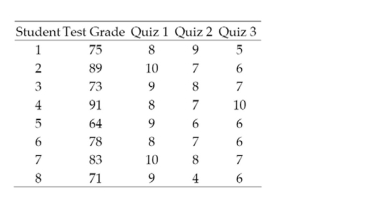The professor would like to use the data to find a first-order model that he might use to predict a student's grade on the first test using that student's grades on the first three quizzes. a. Identify the dependent and independent variables for the model. b. What is the least squares prediction equation? c. Find the SSE and the estimator of $\sigma ^ { 2 }$ for the model.

Which equation represents a complete second-order model for two quantitative independent variables?

Residual analysis can be used to check for violations of the assumptions that the distribution of the random error component is normally distributed with mean 0.

Probabilistic models that include more than one dependent variable are called multiple regression models.

If when using the model $E ( y ) = \beta _ { 0 } + \beta _ { 1 } x _ { 1 } + \beta _ { 2 } x _ { 2 } + \beta _ { 3 } x _ { 1 } x _ { 2 }$ we determine that interaction between $x _ { 1 }$ and $x _ { 2 }$ is not significant, we can drop the $x _ { 1 } x _ { 2 }$ term from the model and use the simpler model $E ( y ) = \beta _ { 0 } + \beta _ { 1 } x _ { 1 } + \beta _ { 2 } x _ { 2 }$ .

A certain type of rare gem serves as a status symbol for many of its owners. In theory, for low prices, the demand decreases as the price of the gem increases. However, experts hypothesize that When the gem is valued at very high prices, the demand increases with price due to the status the Owners believe they gain by obtaining the gem. Thus, the model proposed to best explain the Demand for the gem by its price is the quadratic model $E ( y ) = \beta _ { 0 } + \beta _ { 1 } x + \beta _ { 2 } x ^ { 2 }$ where $y =$ Demand (in thousands) and $x =$ Retail price per carat (dollars). This model was fit to data collected for a sample of 12 rare gems. PARAMETER T for HO: VARIABLES ESTIMATES STD. ERROR PARAMETER =0 PR >|| INTERPCEP 286.42 9.66 29.64 .0001 -.31 .06 -5.14 .0006 \cdot .000067 .00007 .95 .3647 Does there appear to be upward curvature in the response curve relating $y$ (demand) to $x$ (retail price)?

Twenty colleges each recommended one of its graduating seniors for a prestigious graduate fellowship. The process to determine which student will receive the fellowship includes several interviews. The gender of each student and his or her score on the first interview are shown below. 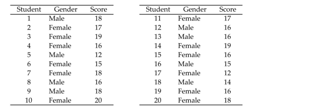a. Suppose you want to use gender to model the score on the interview $y$ . Create the appropriate number of dummy variables for gender and write the model. b. Fit the model to the data. c. Give the null hypothesis for testing whether gender is a useful predictor of the score $y$ . d. Conduct the test and give the appropriate conclusion. Use $\alpha = .05$ .

An elections officer wants to model voter turnout (y)in a precinct as a function of type of election, national or state. Write a model for mean voter turnout, $E ( y )$ , as a function of type of election.

The stepwise regression procedure may not be used when the inclusion of one or more dummy variables is under consideration.

An elections officer wants to model voter turnout (y)in a precinct as a function of the type of precinct. Consider the model relating mean voter turnout, $E ( y )$ , to precinct type: 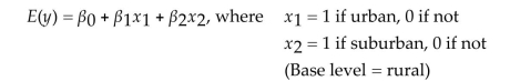Interpret the value of $\beta _ { 0 }$ .

The sum of squared errors (SSE)of a least squares regression model decreases when new terms are added to the model.

Consider the model $y = \beta _ { 0 } + \beta _ { 1 } x _ { 1 } + \beta _ { 2 } x _ { 1 } ^ { 2 } + \beta _ { 3 } x _ { 2 } + \beta _ { 4 } x _ { 3 } + \beta _ { 5 } x _ { 1 } x _ { 2 } + \beta _ { 6 } x _ { 1 } x _ { 3 } + \beta _ { 7 } x _ { 1 } ^ { 2 } x _ { 2 } + \beta _ { 8 } 1 ^ { 2 } x _ { 3 } + \varepsilon$ where $x _ { 1 }$ is a quantitative variable and $x _ { 2 }$ and $x _ { 3 }$ are dummy variables describing a qualitative variable at three levels using the coding scheme $x _ { 2 } = \left\{ \begin{array} { l l } 1 & \text { if level } 2 \\ 0 & \text { otherwise } \end{array} \quad x _ { 3 } = \left\{ \begin{array} { l l } 1 & \text { if level } 3 \\ 0 & \text { otherwise } \end{array} \right. \right.$ The resulting least squares prediction equation is $\hat { y } = 8.8 - 1.1 x _ { 1 } + 3.2 x _ { 1 } ^ { 2 } + 1.6 x _ { 2 } - 4.4 x _ { 3 } + .02 x _ { 1 } x _ { 2 } + 1.3 x _ { 1 } x _ { 3 } + .01 x _ { 1 } ^ { 2 } x _ { 2 } - .06 x _ { 1 } ^ { 2 } x _ { 3 }$ What is the equation of the response curve for $E ( y )$ when $x _ { 2 } = 0$ and $x _ { 3 } = 0$ ?

Operations managers often use work sampling to estimate how much time workers spend on each operation. Work sampling-which involves observing workers at random points in time-was Applied to the staff of the catalog sales department of a clothing manufacturer. The department Applied regression to the following data collected for 40 consecutive working days: 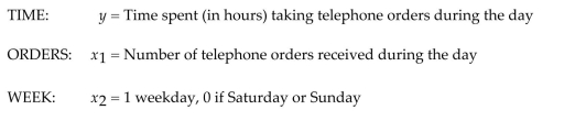Consider the following 2 models: Model 1: $E ( \mathrm { y } ) = \beta _ { 0 } + \beta _ { 1 } x _ { 1 } + \beta _ { 2 } \left( \mathrm { x } _ { 1 } \right) ^ { 2 } + \beta _ { 3 } x _ { 2 } + \beta _ { 4 } x _ { 1 } x _ { 2 } + \beta _ { 5 } \left( x _ { 1 } \right) ^ { 2 } x _ { 2 }$ Model 2: $E ( \mathrm { y } ) = \beta _ { 0 } + \beta _ { 1 } x _ { 1 } + \beta _ { 3 } x _ { 2 }$ What strategy should you employ to decide which of the two models, the higher-order model or the simple linear model, is better?

The complete second-order model with two quantitative independent variables does not allow for interaction between the two independent variables.