Exam 12: Multiple Regression and Model Building
Exam 1: Statistics, Data, and Statistical Thinking77 Questions
Exam 2: Methods for Describing Sets of Data187 Questions
Exam 3: Probability284 Questions
Exam 4: Discrete Random Variables134 Questions
Exam 5: Continuous Random Variables138 Questions
Exam 6: Sampling Distributions52 Questions
Exam 7: Inferences Based on a Single Sample: Estimation With Confidence Intervals125 Questions
Exam 8: Inferences Based on a Single144 Questions
Exam 9: Inferences Based on Two Samples: Confidence Intervals and Tests of Hypotheses100 Questions
Exam 10: Analysis of Variance: Comparing More Than Two Means91 Questions
Exam 11: Simple Linear Regression113 Questions
Exam 12: Multiple Regression and Model Building131 Questions
Exam 13: Categorical Data Analysis60 Questions
Exam 14: Nonparametric Statistics Available Online87 Questions
Select questions type
Consider the second-order model
If is held fixed at , describe the relationship between and .
(Multiple Choice)
4.8/5  (38)
(38)
When modeling E(y)with a single qualitative independent variable, the number of 0-1 dummy
variables in the model is equal to the number of levels of the qualitative variable.
(True/False)
4.9/5 (28)
A study of the top MBA programs attempted to predict the average starting salary (in 's) of graduates of the program based on the amount of tuition (in 's) charged by the program and the average GMAT score of the program's students. The results of a regression analysis based on a sample of 75 MBA programs is shown below:
Least Squares Linear Regression of Salary
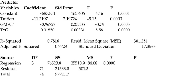 Cases Included Missing Cases 0
One of the -test test statistics is shown on the printout to be the value . Interpret this value.
Cases Included Missing Cases 0
One of the -test test statistics is shown on the printout to be the value . Interpret this value.
(Multiple Choice)
4.9/5 (39)
The table shows the profit y (in thousands of dollars)that a company made during a
month when the price of its product was x dollars per unit. Profit, y Price, x 12 1.20 17 1.25 20 1.29 21 1.30 24 1.35 26 1.39 27 1.40 23 1.45 21 1.49 20 1.50 15 1.55 11 1.59 10 1.60 5 1.65
a. Fit the model to the data and give the least squares prediction equation.
b. Plot the fitted equation on a scattergram of the data.
c. Is there sufficient evidence of downward curvature in the relationship between profit and price? Use .
(Essay)
4.8/5 (36)
In an interaction model, the relationship between and is linear for each fixed value of but the slopes of the lines relating and may be different for two different fixed values of .
(True/False)
4.7/5 (43)
The method of fitting first-order models is the same as that of fitting the simple straight-line
model, i.e. the method of least squares.
(True/False)
4.9/5 (40)
It is desired to build a regression model to predict the sales price of a single family home, based on the size of the house and the neighborhood the home is located in. The goal is to compare the prices of homes that are located in two different neighborhoods. A complete 2nd-order model is proposed. Which regression model proposes the complete 2nd-order model?
(Multiple Choice)
4.8/5 (38)
The table below shows data for n = 20 observations. y x1 x2 18 3 8 23 5 10 15 2 7 31 6 12 24 4 9 28 5 11 17 2 7 19 3 8 30 7 10 28 5 8 14 3 6 32 7 11 17 2 8 24 5 10 26 6 11 27 6 11 21 3 6 31 7 13 19 2 8 25 5 10
a. Use a first-order regression model to find a least squares prediction equation for the model.
b. Find a confidence interval for the coefficient of in your model. Interpret the result.
c. Find a confidence interval for the coefficient of in your model. Interpret the result.
d. Find and and interpret these values.
e. Test the null hypothesis against the alternative hypothesis : at least one . Use . Interpret the result.
(Essay)
4.9/5 (44)
The printout below shows part of the least squares regression analysis for the model fit to a set of data. The model attempts to predict a score on the final exam in a statistics course based on the scores on the first two tests in the class.
ANOVA
df SS MS F Significance F Regression 2 1293.125328 646.5626641 21.27366772 2.35769-05 Residual 17 516.6746719 30.39262776 Total 19 1809.8
Coefficients Standard Error t Stat P-value Lower 95\% Upper 95\% Intercept -4.409686163 16.72267106 -0.263695085 0.795184685 -39.69148734 30.87211502 Test 1 0.397435806 0.343012569 1.158662514 0.262611745 -0.326258467 1.121130079 Test 2 0.638805278 0.224623383 2.843894834 0.011217936 0.164890704 1.112719852
Is there evidence of multicollinearity in the printout? Explain.
(Essay)
4.8/5 (34)
A study of the top MBA programs attempted to predict the average starting salary (in $1000ʹs)of graduates of the program based on the amount of tuition (in $1000ʹs)charged by the program and
The average GMAT score of the programʹs students. The results of a regression analysis based on a
Sample of 75 MBA programs is shown below: Least Squares Linear Regression of Salary
 The global-f test statistic is shown on the printout to be the value . Interpret this value.
(Multiple Choice)
4.9/5 (31)
As part of a study at a large university, data were collected on n = 224 freshmen computer science (CS)majors in a particular year. The researchers were interested in modeling y, a studentʹs grade
Point average (GPA)after three semesters, as a function of the following independent variables
(recorded at the time the students enrolled in the university): average high school grade in mathematics (HSM)
average high school grade in science (HSS)
average high school grade in English (HSE)
SAT mathematics score (SATM)
SAT verbal score (SATV)
A first-order model was fit to data with the following results:
SOURCE DF SS MS FVALUE PROB >F MODEL 5 28.64 5.73 11.69 .0001 ERROR 218 106.82 0.49 TOTAL 223 135.46
ROOT MSE 0.700 R-SQUARE 0.211 DEP MEAN 4.635 ADJ R-SQ 0.193
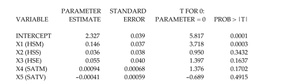 Interpret the value under the column heading .
(Multiple Choice)
5.0/5 (46)
A collector of grandfather clocks believes that the price received for the clocks at an auction increases with the number of bidders, but at an increasing (rather than a constant)rate. Thus, the
Model proposed to best explain auction price (y, in dollars)by number of bidders (x)is the
Quadratic model
This model was fit to data collected for a sample of 32 clocks sold at auction; a portion of the printout follows:
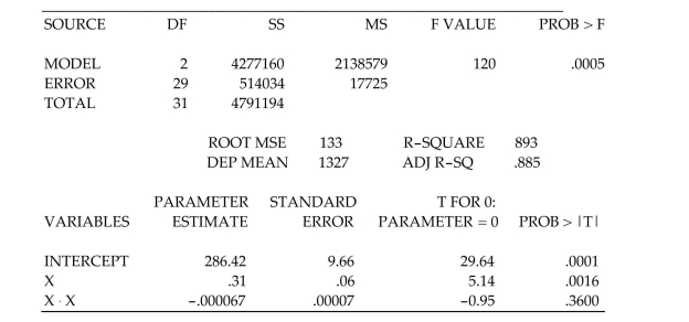 An outlier for the model is a clock with a residual that in absolute value. (Fill in the blank.)
(Multiple Choice)
4.8/5 (28)
When using the model for one qualitative independent variable with a coding convention, represents the difference between the mean responses for the level assigned the value 1 and the base level.
(True/False)
5.0/5 (40)
Consider the interaction model . Determine the change in when is changed from 6 to 7 and is held fixed at 3 .
(Multiple Choice)
4.9/5 (42)
As part of a study at a large university, data were collected on n = 224 freshmen computer science (CS)majors in a particular year. The researchers were interested in modeling y, a studentʹs grade
Point average (GPA)after three semesters, as a function of the following independent variables
(recorded at the time the students enrolled in the university): average high school grade in mathematics (HSM)
average high school grade in science (HSS)
average high school grade in English (HSE)
SAT mathematics score (SATM)
SAT verbal score (SATV)
A first-order model was fit to data.
Give the null hypothesis for testing the overall adequacy of the model.
(Multiple Choice)
4.9/5 (31)
During its manufacture, a product is subjected to four different tests in sequential order. An efficiency expert claims that the fourth (and last) test is unnecessary since its results can be predicted based on the first three tests. To test this claim, multiple regression will be used to model Test4 score , as a function of Test1 score , Test 2 score , and Test3 score ( . [Note: All test scores range from 200 to 800 , with higher scores indicative of a higher quality product.] Consider the model:
The first-order model was fit to the data for each of 12 units sampled from the production line.
A prediction interval for Test4 score of a product with Test1 , Test , and Test3 is . Interpret this result.
(Multiple Choice)
4.8/5 (31)
A term that contains the value of a quantitative variable raised to the second power is called a
higher-order term.
(True/False)
4.8/5 (28)
A certain type of rare gem serves as a status symbol for many of its owners. In theory, for
low prices, the demand decreases as the price of the gem increases. However, experts
hypothesize that when the gem is valued at very high prices, the demand increases with
price due to the status the owners believe they gain by obtaining the gem. Thus, the model
proposed to best explain the demand for the gem by its price is the quadratic model
where Demand (in thousands) and Retail price per carat (dollars).
This model was fit to data collected for a sample of 12 rare gems. A portion of the printout is given below:
SOURCE DF SS MS F PR > F Model 2 115145 57573 373 .0001 Error 9 1388 154 TOTAL 11 116533
Root MSE 12.42 R-Square .988 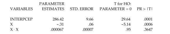 Is there sufficient evidence to indicate the model is useful for predicting the demand for the gem? Use .
(Essay)
4.9/5 (47)
Once interaction has been established between and , the first-order terms for and may be deleted from the regression model leaving the higher-order term containing the product of and .
(True/False)
4.8/5 (44)
Filters
- Essay(0)
- Multiple Choice(0)
- Short Answer(0)
- True False(0)
- Matching(0)