It is believed that the sales volume of one-liter Pepsi bottles depends on the price of the bottle and the price of a one-liter bottle of Coca-Cola. The following data have been collected for a certain sales region. The linear model Pepsi Sales = β0 + β1Pepsi Price + β2Cola Price + ε and the log-log model ln(Pepsi Sales) = β0 + β1ln(Pepsi Price) + β2ln(Cola Price) + ε have been estimated as follows: Discuss the choice between the linear model and the log-log model.

Both models, Pepsi Sales = β 0 + β 1 Pepsi Pr

In the model ln(y) = β0 + β1 ln(x) + ε, the coefficient β1 is the approximate ________.

A) change in E(y) when x increases by one unit B) percentage change in E(y) when x increases by 1% C) percentage change in E(y) when x increases by one unit D) change in E(y) when x increases by 1% A) change in E(y) when x increases by one unit B) percentage change in E(y) when x increases by 1% C) percentage change in E(y) when x increases by one unit D) change in E(y) when x increases by 1%

For the quadratic regression equation = b0 + b1x + b2x2, the optimum (maximum or minimum) value of is ________.

A) -b1/2b2 B) b1/2b2 C) b0 - D) b0 - A) -b1/2b2 B) b1/2b2 C) b0 - D) b0 -

Exam 16: Regression Models for Nonlinear Relationships

For the quadratic regression model = b₀ + b₁x + b₂x², b₁ can be interpreted as the change in the predicted value of y when x increases by 1 unit.

(True/False)

4.8/5

(31)

Question 101

It is believed that the sales volume of one-liter Pepsi bottles depends on the price of the bottle and the price of a one-liter bottle of Coca-Cola. The following data have been collected for a certain sales region. 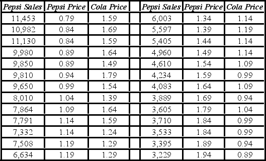The linear model Pepsi Sales = β₀ + β₁Pepsi Price + β₂Cola Price + ε and the log-log model ln(Pepsi Sales) = β₀ + β₁ln(Pepsi Price) + β₂ln(Cola Price) + ε have been estimated as follows: Discuss the choice between the linear model and the log-log model.

(Essay)

4.8/5

(36)

Question 102

Thirty employed single individuals were randomly selected to examine the relationship between their age (Age) and their credit card debt (Debt) expressed as a percentage of their annual income. Three polynomial models were applied and the following table summarizes Excel's regression results. Suppose the restriction β₃ = 0 is imposed on the cubic regression model Debt = β₀+ β₁Age + β₂Age²^{+ β}₃Age³+ ε. What regression equation is obtained under this restriction?

(Essay)

4.8/5

(31)

Question 103

Thirty employed single individuals were randomly selected to examine the relationship between their age (Age) and their credit card debt (Debt) expressed as a percentage of their annual income. Three polynomial models were applied and the following table summarizes Excel's regression results. Using the quadratic regression equation, find the predicted maximum percentage debt.

(Short Answer)

5.0/5

(35)

Question 104

The regression model ln(y) = β₀ + β₁ln(x) + ε is called a log-log model.

(True/False)

4.9/5

(44)

Question 105

For the log-log model ln(y) = β₀ + β₁ln(x) + ε, β₁ is the approximate percent change in E(y) when x increases by 1%.

(True/False)

4.8/5

(34)

Question 106

The following data show the demand for an airline ticket dependent on the price of this ticket. 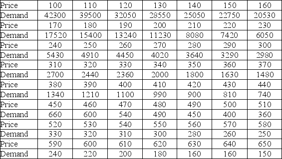For the assumed cubic and log-log regression models, Demand = β₀ + β₁Price + β₂Price²+ β₃Price³+ ε and ln(Demand) = β₀ + β₁ln(Price) + ε, the following regression results are available. Assuming that the sample correlation coefficient between Demand and = exp(26.3660 - 3.2577 ln(Price) + (0.2071)²/2) is 0.956, what is the predicted demand for a price of $250 found by the model with better fit?

(Multiple Choice)

4.8/5

(37)

Question 107

In the model ln(y) = β₀ + β₁ ln(x) + ε, the coefficient β₁ is the approximate ________.

(Multiple Choice)

4.9/5

(38)

Question 108

Typically, the sales volume declines with an increase of a product price. It has been observed, however, that for some luxury goods the sales volume may increase when the price increases. The following scatterplot illustrates this rather unusual relationship. 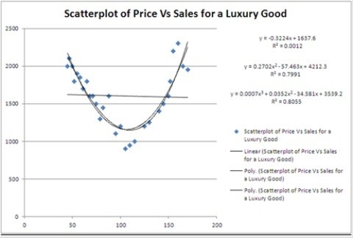Which of the following models is most likely to be chosen in order to describe the relationship between Price and Sales?

(Multiple Choice)

4.8/5

(36)

Question 109

The following data, with the corresponding Excel scatterplot, show the average growth rate of Weeping Higan cherry trees planted in Washington, DC. At the time of planting, the trees were one year old and were all six feet in height. 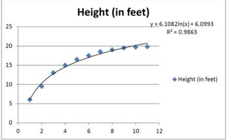Which of the following is the predicted height of an eight-year-old cherry tree that was planted as a one-year-old and six-foot-tall tree?

(Multiple Choice)

4.9/5

(29)

Question 110

It is believed that the sales volume of one-liter Pepsi bottles depends on the price of the bottle and the price of a one-liter bottle of Coca-Cola. The following data have been collected for a certain sales region. The linear model Pepsi Sales = β₀ + β₁Pepsi Price + β₂Cola Price + ε and the log-log model ln(Pepsi Sales) = β₀ + β₁ln(Pepsi Price) + β₂ln(Cola Price) + ε have been estimated as follows: 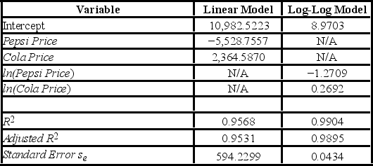For log-log model, interpret the estimated coefficient for ln(Cola Price).

(Essay)

4.9/5

(32)

Question 111

The following scatterplot shows productivity and number hired workers with a fitted quadratic regression model. 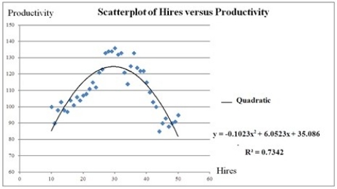For which value of Hires is the predicted Productivity maximized? Note: Do not round to the nearest integer.

(Multiple Choice)

4.8/5

(29)

Question 112

Thirty employed single individuals were randomly selected to examine the relationship between their age (Age) and their credit card debt (Debt) expressed as a percentage of their annual income. Three polynomial models were applied and the following table summarizes Excel's regression results. What is the percentage of variations in Debt explained by the regression model that provides the best fit?

(Short Answer)

4.8/5

(37)

Question 113

The log-log and exponential models, ln(x) = β₀ + β₁ln(x) + ε and ln(y) = β₀ + β₁x + ε, were fit given data on y and x, and the following table summarizes the regression results. Which of the two models provides a better fit?

(Multiple Choice)

4.8/5

(34)

Question 114

When not all variables are transformed with logarithms, the models are called ________ models.

(Short Answer)

4.8/5

(36)

Question 115

The following scatterplot shows productivity and number hired workers with a fitted quadratic regression model. 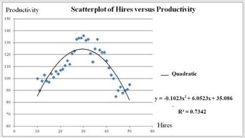Assuming that the number of hired workers must be an integer, what is the maximum productivity predicted by the model?

(Multiple Choice)

4.8/5

(42)

Question 116

The following scatterplot shows productivity and number hired workers with a fitted quadratic regression model. 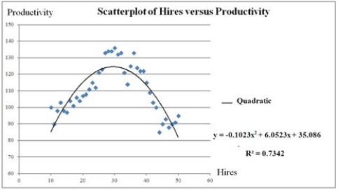Assuming that the number of hired workers must be integer, how many workers should be hired to achieve the highest productivity according to the model?

(Multiple Choice)

4.9/5

(36)

Question 117

For the quadratic regression equation = b₀ + b₁x + b₂x², the optimum (maximum or minimum) value of is ________.

(Multiple Choice)

4.9/5

(38)

Question 118

Showing 101 - 118 of 118

For the quadratic regression model = b₀ + b₁x + b₂x², b₁ can be interpreted as the change in the predicted value of y when x increases by 1 unit.

The regression model ln(y) = β₀ + β₁ln(x) + ε is called a log-log model.

For the log-log model ln(y) = β₀ + β₁ln(x) + ε, β₁ is the approximate percent change in E(y) when x increases by 1%.

In the model ln(y) = β₀ + β₁ ln(x) + ε, the coefficient β₁ is the approximate ________.

The following scatterplot shows productivity and number hired workers with a fitted quadratic regression model. For which value of Hires is the predicted Productivity maximized? Note: Do not round to the nearest integer.

The log-log and exponential models, ln(x) = β₀ + β₁ln(x) + ε and ln(y) = β₀ + β₁x + ε, were fit given data on y and x, and the following table summarizes the regression results. Which of the two models provides a better fit?

When not all variables are transformed with logarithms, the models are called ________ models.

The following scatterplot shows productivity and number hired workers with a fitted quadratic regression model. Assuming that the number of hired workers must be an integer, what is the maximum productivity predicted by the model?

The following scatterplot shows productivity and number hired workers with a fitted quadratic regression model. Assuming that the number of hired workers must be integer, how many workers should be hired to achieve the highest productivity according to the model?

For the quadratic regression equation = b₀ + b₁x + b₂x², the optimum (maximum or minimum) value of is ________.

Statistics and Data

Tabular and Graphical Methods

Numerical Descriptive Measures

Introduction to Probability

Discrete Probability Distributions

Continuous Probability Distributions

Sampling and Sampling Distributions

Interval Estimation

Hypothesis Testing

Statistical Inference Concerning Two Populations

Statistical Inference Concerning Variance

Chi-Square Tests

Analysis of Variance

Regression Analysis

Inference With Regression Models

Regression Models With Dummy Variables

Time Series and Forecasting

Returns, Index Numbers, and Inflation

Nonparametric Tests

Filters

Exam 16: Regression Models for Nonlinear Relationships

For the quadratic regression model = b0 + b1x + b2x2, b1 can be interpreted as the change in the predicted value of y when x increases by 1 unit.

The regression model ln(y) = β0 + β1ln(x) + ε is called a log-log model.

For the log-log model ln(y) = β0 + β1ln(x) + ε, β1 is the approximate percent change in E(y) when x increases by 1%.

In the model ln(y) = β0 + β1 ln(x) + ε, the coefficient β1 is the approximate ________.

The following scatterplot shows productivity and number hired workers with a fitted quadratic regression model. For which value of Hires is the predicted Productivity maximized? Note: Do not round to the nearest integer.

The log-log and exponential models, ln(x) = β0 + β1ln(x) + ε and ln(y) = β0 + β1x + ε, were fit given data on y and x, and the following table summarizes the regression results. Which of the two models provides a better fit?

When not all variables are transformed with logarithms, the models are called ________ models.

The following scatterplot shows productivity and number hired workers with a fitted quadratic regression model. Assuming that the number of hired workers must be an integer, what is the maximum productivity predicted by the model?

The following scatterplot shows productivity and number hired workers with a fitted quadratic regression model. Assuming that the number of hired workers must be integer, how many workers should be hired to achieve the highest productivity according to the model?

For the quadratic regression equation = b0 + b1x + b2x2, the optimum (maximum or minimum) value of is ________.

Statistics and Data

Tabular and Graphical Methods

Numerical Descriptive Measures

Introduction to Probability

Discrete Probability Distributions

Continuous Probability Distributions

Sampling and Sampling Distributions

Interval Estimation

Hypothesis Testing

Statistical Inference Concerning Two Populations

Statistical Inference Concerning Variance

Chi-Square Tests

Analysis of Variance

Regression Analysis

Inference With Regression Models

Regression Models With Dummy Variables

Time Series and Forecasting

Returns, Index Numbers, and Inflation

Nonparametric Tests

Filters

For the quadratic regression model = b₀ + b₁x + b₂x², b₁ can be interpreted as the change in the predicted value of y when x increases by 1 unit.

The regression model ln(y) = β₀ + β₁ln(x) + ε is called a log-log model.

For the log-log model ln(y) = β₀ + β₁ln(x) + ε, β₁ is the approximate percent change in E(y) when x increases by 1%.

In the model ln(y) = β₀ + β₁ ln(x) + ε, the coefficient β₁ is the approximate ________.

The log-log and exponential models, ln(x) = β₀ + β₁ln(x) + ε and ln(y) = β₀ + β₁x + ε, were fit given data on y and x, and the following table summarizes the regression results. Which of the two models provides a better fit?

For the quadratic regression equation = b₀ + b₁x + b₂x², the optimum (maximum or minimum) value of is ________.