Question 1

The quadratic regression model allows for one change in ________.

Accepted Answer

The answer of The quadratic regression model allows for one...

Question 2

The quadratic regression model   = b0 + b1x + b2x2 allows for one sign change in the slope capturing the influence of x on y.

Accepted Answer

A) True 
 B)False

Question 3

In which of the following models does the slope coefficient b1 measure the change in   when x increases by one unit?

Accepted Answer

A)  Linear regression model 
B)  Exponential regression model 
C)  Logarithmic regression model 
D)  Log-log regression model 
A)  Linear regression model 
B)  Exponential regression model 
C)  Logarithmic regression model 
D)  Log-log regression model

Question 4

The fit of the models y = β0 + β1x + ε and y = β0 + β1ln(x) + ε can be compared using the coefficient of determination R2.

Accepted Answer

A) True 
 B)False

Question 5

A quadratic regression model is a polynomial regression model of order 2.

Accepted Answer

A) True 
 B)False

Question 6

The following data show the demand for an airline ticket dependent on the price of this ticket. 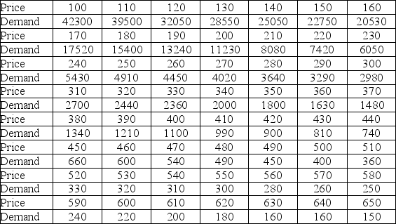  For the assumed cubic and log-log regression models, Demand = β0 + β1Price + β2Price2 + β3Price3 + ε and ln(Demand) = β0 + β1ln(Price) + ε, the following regression results are available.   Which of the following does the slope of the obtained log-log regression equation ln (   ) = 26.3660 - 3.2577 ln(Price) signify?

Accepted Answer

A)  For every 1% increase in the price, the predicted demand declines by approximately 3.2577%. 
B)  For every 1% increase in the demand, the expected price increases by approximately 3.2577%. 
C)  For every 1% increase in the demand, the expected price decreases by approximately 3.2577%. 
D)  For every 1% increase in the price, the predicted demand increases by approximately 3.2577%. 
A)  For every 1% increase in the price, the predicted demand declines by approximately 3.2577%. 
B)  For every 1% increase in the demand, the expected price increases by approximately 3.2577%. 
C)  For every 1% increase in the demand, the expected price decreases by approximately 3.2577%. 
D)  For every 1% increase in the price, the predicted demand increases by approximately 3.2577%.

Question 7

Thirty employed single individuals were randomly selected to examine the relationship between their age (Age) and their credit card debt (Debt) expressed as a percentage of their annual income. Three polynomial models were applied and the following table summarizes Excel's regression results.   What is the value of the test statistic for testing H0: β2 = β3 = 0 against HA: β2 ≠ 0 or β3 ≠ 0 in the model Debt = β0 + β1Age + β2Age2+ β3Age3 + ε?

Accepted Answer

Question 8

It is believed that the sales volume of one-liter Pepsi bottles depends on the price of the bottle and the price of a one-liter bottle of Coca-Cola. The following data have been collected for a certain sales region. 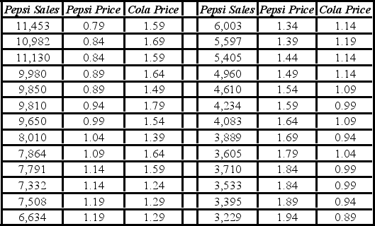  The linear model Pepsi Sales = β0 + β1Pepsi Price + β2Cola Price + ε and the log-log model ln(Pepsi Sales) = β0 + β1ln(Pepsi Price) + β2ln(Cola Price) + ε have been estimated as follows:  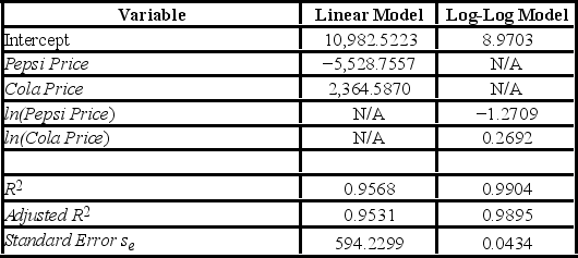 Using the linear model, calculate the predicted Pepsi Sales when the Pepsi Price is $1.50 and the Cola Price is $1.25.

Accepted Answer

Question 9

The following data show the cooling temperatures of a freshly brewed cup of coffee after it is poured from the brewing pot into a serving cup. The brewing pot temperature is approximately 180º F.   The output for an exponential model, ln(Temp) = β0 + β1Time + ε, t is below.   How many minutes must elapse after the brewing in order to cool the coffee to 158°F?

Accepted Answer

A)  About five minutes 
B)  About six minutes 
C)  About seven minutes 
D)  About eight minutes 
A)  About five minutes 
B)  About six minutes 
C)  About seven minutes 
D)  About eight minutes

Question 10

The scatterplot shown below represents a typical shape of a cubic regression model y = β0 + β1x + β2x2 + β3x3 + ε. 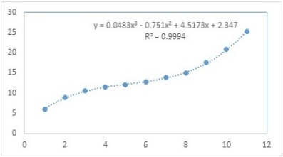  Which of the following is true about values of the regression coefficients?

Accepted Answer

A)  β1 > 0; β2 > 0; β3 > 0 
B)  β1 2 > 0; β3 > 0 
C)  β1 2 3 > 0 
D)  β1 > 0; β2 3 > 0 
A)  β1 > 0; β2 > 0; β3 > 0 
B)  β1 2 > 0; β3 > 0 
C)  β1 2 3 > 0 
D)  β1 > 0; β2 3 > 0

Question 11

The following data show the cooling temperatures of a freshly brewed cup of coffee after it is poured from the brewing pot into a serving cup. The brewing pot temperature is approximately 180º F. 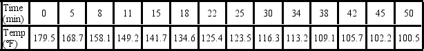  The output for an exponential model, ln(Temp) = β0 + β1Time + ε, t is below.   Which of the following is the standard error of the estimate?

Accepted Answer

A)  0.03421 
B)  0.45476 
C)  0.00117 
D)  0.67436 
A)  0.03421 
B)  0.45476 
C)  0.00117 
D)  0.67436

Question 12

Thirty employed single individuals were randomly selected to examine the relationship between their age (Age) and their credit card debt (Debt) expressed as a percentage of their annual income. Three polynomial models were applied and the following table summarizes Excel's regression results.   What is the sample correlation coefficient between Age and Debt?

Accepted Answer

The answer of Thirty employed single individuals were randomly selected...

Question 13

The following data show the demand for an airline ticket dependent on the price of this ticket.   For the assumed cubic and log-log regression models, Demand = β0 + β1Price + β2Price2 + β3Price3 + ε and ln(Demand) = β0 + β1ln(Price) + ε, the following regression results are available.   Which of the following is the percentage of variation in ln(Demand) explained by the log-log regression model?

Accepted Answer

A)  98.52% 
B)  98.50% 
C)  91.39% 
D)  97.93% 
A)  98.52% 
B)  98.50% 
C)  91.39% 
D)  97.93%

Question 14

The following data show the cooling temperatures of a freshly brewed cup of coffee after it is poured from the brewing pot into a serving cup. The brewing pot temperature is approximately 180º F.   The output for an exponential model, ln(Temp) = β0 + β1Time + ε, is below.   Which of the following is the regression equation for making predictions concerning the coffee temperature?

Accepted Answer

A)    = exp (5.1444 - 0.0118Time 
B)    = exp (5.1450 - 0.0118Time 
C)    = 5.1444 - 0.0118Time 
D)    = 5.1450 - 0.0118Time 
A)    = exp (5.1444 - 0.0118Time 
B)    = exp (5.1450 - 0.0118Time 
C)    = 5.1444 - 0.0118Time 
D)    = 5.1450 - 0.0118Time

Question 15

Typically, the sales volume declines with an increase of a product price. It has been observed, however, that for some luxury goods the sales volume may increase when the price increases. The following scatterplot illustrates this rather unusual relationship. 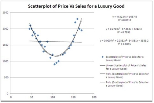  What can be said about the linear relationship between Price and Sales?

Accepted Answer

A)  The relationship is negatively moderate. 
B)  There is no relationship. 
C)  The relationship is positively strong. 
D)  The relationship is negatively strong. 
A)  The relationship is negatively moderate. 
B)  There is no relationship. 
C)  The relationship is positively strong. 
D)  The relationship is negatively strong.

Question 16

The quadratic and logarithmic models, y = β0 + β1x + β2x2 + ε and y = β0 + β1 ln(x) + ε, were fit given data on y and x, and the following table summarizes the regression results. Which of the two models provides a better fit?

Accepted Answer

A)  The quadratic model. 
B)  The logarithmic model. 
C)  The models are not comparable. 
D)  The provided information is not sufficient to make the conclusion. 
A)  The quadratic model. 
B)  The logarithmic model. 
C)  The models are not comparable. 
D)  The provided information is not sufficient to make the conclusion.

Question 17

The following data show the cooling temperatures of a freshly brewed cup of coffee after it is poured from the brewing pot into a serving cup. The brewing pot temperature is approximately 180º F.   The output for an exponential model ln(Temp) = β0 + β1Time + ε, t is below.   Which of the following is the percentage of variation in ln(Temp) explained by the model?

Accepted Answer

A)  45.48% 
B)  97.01% 
C)  1.40% 
D)  46.88% 
A)  45.48% 
B)  97.01% 
C)  1.40% 
D)  46.88%

Question 18

The following data show the cooling temperatures of a freshly brewed cup of coffee after it is poured from the brewing pot into a serving cup. The brewing pot temperature is approximately 180º F.   The output for an exponential model, ln(Temp) = β0 + β1Time + ε, is below.   During one minute, the predicted temperature decreases by approximately ________.

Accepted Answer

A)  0.0118° F 
B)  1.18° F 
C)  1.18% 
D)  11.8% 
A)  0.0118° F 
B)  1.18° F 
C)  1.18% 
D)  11.8%

Question 19

The following data show the demand for an airline ticket dependent on the price of this ticket.   For the assumed cubic and log-log regression models, Demand = β0 + β1Price + β2Price2 + β3Price3 + ε and ln(Demand) = β0 + β1ln(Price) + ε, the following regression results are available.   Assuming that the sample correlation coefficient between Demand and   = exp(26.3660 - 3.2577 ln(Price) + (0.2071)2/2) is 0.956, what is the percentage of variations in Demand explained by the log-log regression model?

Accepted Answer

A)  98.52% 
B)  98.50% 
C)  91.39% 
D)  97.93% 
A)  98.52% 
B)  98.50% 
C)  91.39% 
D)  97.93%

Question 20

Thirty employed single individuals were randomly selected to examine the relationship between their age (Age) and their credit card debt (Debt) expressed as a percentage of their annual income. Three polynomial models were applied and the following table summarizes Excel's regression results.   Using the quadratic regression equation, find the age of an employed single person with the highest predicted percentage debt.

Accepted Answer

The answer of Thirty employed single individuals were randomly selected...

The quadratic regression model allows for one change in ________.

The quadratic regression model = b₀ + b₁x + b₂x² allows for one sign change in the slope capturing the influence of x on y.

In which of the following models does the slope coefficient b₁ measure the change in when x increases by one unit?

The fit of the models y = β₀ + β₁x + ε and y = β₀ + β₁ln(x) + ε can be compared using the coefficient of determination R².

A quadratic regression model is a polynomial regression model of order 2.

The scatterplot shown below represents a typical shape of a cubic regression model y = β₀ + β₁x + β₂x² + β₃x³ + ε. Which of the following is true about values of the regression coefficients?

The quadratic and logarithmic models, y = β₀ + β₁x + β₂x² + ε and y = β₀ + β₁ ln(x) + ε, were fit given data on y and x, and the following table summarizes the regression results. Which of the two models provides a better fit?

Statistics and Data

Tabular and Graphical Methods

Numerical Descriptive Measures

Introduction to Probability

Discrete Probability Distributions

Continuous Probability Distributions

Sampling and Sampling Distributions

Interval Estimation

Hypothesis Testing

Statistical Inference Concerning Two Populations

Statistical Inference Concerning Variance

Chi-Square Tests

Analysis of Variance

Regression Analysis

Inference With Regression Models

Regression Models With Dummy Variables

Time Series and Forecasting

Returns, Index Numbers, and Inflation

Nonparametric Tests

Filters

Exam 16: Regression Models for Nonlinear Relationships

The quadratic regression model allows for one change in ________.

The quadratic regression model = b0 + b1x + b2x2 allows for one sign change in the slope capturing the influence of x on y.

In which of the following models does the slope coefficient b1 measure the change in when x increases by one unit?

The fit of the models y = β0 + β1x + ε and y = β0 + β1ln(x) + ε can be compared using the coefficient of determination R2.

A quadratic regression model is a polynomial regression model of order 2.

The scatterplot shown below represents a typical shape of a cubic regression model y = β0 + β1x + β2x2 + β3x3 + ε. Which of the following is true about values of the regression coefficients?

The quadratic and logarithmic models, y = β0 + β1x + β2x2 + ε and y = β0 + β1 ln(x) + ε, were fit given data on y and x, and the following table summarizes the regression results. Which of the two models provides a better fit?

Statistics and Data

Tabular and Graphical Methods

Numerical Descriptive Measures

Introduction to Probability

Discrete Probability Distributions

Continuous Probability Distributions

Sampling and Sampling Distributions

Interval Estimation

Hypothesis Testing

Statistical Inference Concerning Two Populations

Statistical Inference Concerning Variance

Chi-Square Tests

Analysis of Variance

Regression Analysis

Inference With Regression Models

Regression Models With Dummy Variables

Time Series and Forecasting

Returns, Index Numbers, and Inflation

Nonparametric Tests

Filters

The quadratic regression model = b₀ + b₁x + b₂x² allows for one sign change in the slope capturing the influence of x on y.

In which of the following models does the slope coefficient b₁ measure the change in when x increases by one unit?

The fit of the models y = β₀ + β₁x + ε and y = β₀ + β₁ln(x) + ε can be compared using the coefficient of determination R².

The scatterplot shown below represents a typical shape of a cubic regression model y = β₀ + β₁x + β₂x² + β₃x³ + ε. Which of the following is true about values of the regression coefficients?

The quadratic and logarithmic models, y = β₀ + β₁x + β₂x² + ε and y = β₀ + β₁ ln(x) + ε, were fit given data on y and x, and the following table summarizes the regression results. Which of the two models provides a better fit?