Exam 16: Time Series Forecasting
Exam 1: An Introduction to Business Statistics54 Questions
Exam 2: Descriptive Statistics: Tabular and Graphical Methods90 Questions
Exam 3: Descriptive Statistics: Numerical Methods149 Questions
Exam 4: Probability135 Questions
Exam 5: Discrete Random Variables128 Questions
Exam 6: Continuous Random Variables150 Questions
Exam 7: Sampling and Sampling Distributions116 Questions
Exam 8: Confidence Intervals144 Questions
Exam 9: Hypothesis Testing148 Questions
Exam 10: Statistical Inferences Based on Two Samples132 Questions
Exam 11: Experimental Design and Analysis of Variance115 Questions
Exam 12: Chi-Square Tests96 Questions
Exam 13: Simple Linear Regression Analysis148 Questions
Exam 14: Multiple Regression122 Questions
Exam 15: Model Building and Model Diagnostics102 Questions
Exam 16: Time Series Forecasting150 Questions
Exam 17: Process Improvement Using Control Charts122 Questions
Exam 18: Nonparametric Methods97 Questions
Exam 19: Decision Theory90 Questions
Select questions type
When using simple exponential smoothing,the more recent the time series observation,the _________ its corresponding weight.
(Multiple Choice)
4.9/5  (38)
(38)
A restaurant has been experiencing higher sales during the weekends of compared to the weekdays.Daily restaurant sales patterns for this restaurant over a week are an example of _________ component of time series.
(Multiple Choice)
4.8/5 (40)
A positive autocorrelation implies that negative error terms will be followed by negative error terms.
(True/False)
4.8/5 (35)
 Based on the information given in the table above,what is the MSD?
(Multiple Choice)
4.9/5 (30)
The linear regression trend model was applied to a time series sales data based on the last 24 months' sales.The following partial computer output was obtained. 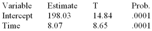 Test the significance of the time term at = .05.State the critical t value and make your decision using a two-sided alternative.
(Essay)
4.8/5 (35)
The price and quantity of several food items are listed below for the years 1990 and 2000. 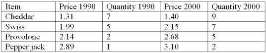 Compute the Laspeyres index using 1990 as the base year.
(Essay)
4.8/5 (31)
Consider the quarterly production data (in thousands of units)for the XYZ manufacturing company below.The normalized (adjusted)seasonal factors are .9982,.9263,1.139,.9365 for winter,spring,summer and fall respectively. 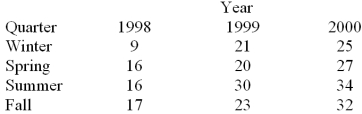 Based on the following deseasonalized observations (dt)given below,a trend line was estimated.
 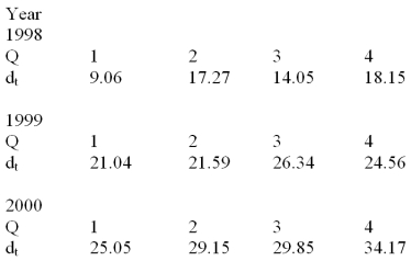 The following MINITAB output gives the straight-line trend equation fitted to the deseasonalized observations.Based on the trend equation given below,calculate the trend value for each period in the time series.
The regression equation is
Deseasonalized = 10.1 + 1.91 Time
The following MINITAB output gives the straight-line trend equation fitted to the deseasonalized observations.Based on the trend equation given below,calculate the trend value for each period in the time series.
The regression equation is
Deseasonalized = 10.1 + 1.91 Time 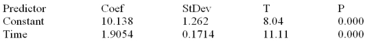
(Essay)
5.0/5 (45)
 Based on the information given in the table above,what is the MAD?
(Multiple Choice)
4.7/5 (45)
The upward or downward movement that characterizes a time series over a period of time is referred to as ____.
(Multiple Choice)
4.9/5 (38)
Consider the quarterly production data (in thousands of units)for the XYZ manufacturing company below.The normalized (adjusted)seasonal factors are .9982,.9263,1.139,.9365 for winter,spring,summer and fall respectively. 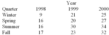 Based on the following deseasonalized observations (dt)given below,a trend line was estimated.The linear regression trend equation is: trt = 10.1 + 1.91 (t).Use the forecasting equation
  and calculate the forecasted demand for the fall quarter of 1998 and summer quarter of 2000.
(Essay)
4.7/5 (39)
If a time series exhibits increasing seasonal variation,one approach is to first use a ______________ transformation that produces a transformed time series that exhibits constant seasonal variation.Then,_________ variables can be used to model the time series with constant seasonal variation.
(Multiple Choice)
4.9/5 (35)
In the multiplicative decomposition method,the centered moving averages provide an estimate of trend x _____.
(Multiple Choice)
4.8/5 (34)
The linear regression trend model was applied to a time series sales data based on the last 24 months' sales.The following partial computer output was obtained. 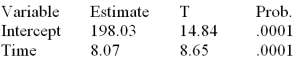 Write the prediction equation.
(Essay)
4.8/5 (31)
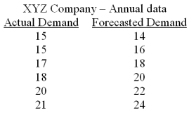
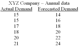
Two forecasting models were used to predict the future values of a time series.The forecasts are shown below with the actual values: 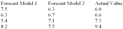 Calculate the mean squared deviation (MSD)for Model 1.
(Essay)
4.9/5 (39)
Which of the following time series forecasting methods would not be used to forecast seasonal data?
(Multiple Choice)
5.0/5 (42)
The linear regression trend model was applied to a time series of sales data based on the last 16 months of sales.The following partial computer output was obtained: 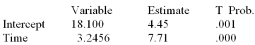 Write the prediction equation.
(Essay)
4.9/5 (38)
When there is first-order autocorrelation,the error term in period t is related to the error term in period _____.
(Multiple Choice)
4.8/5 (41)
When a forecaster uses the _________________ method she or he assumes that the time series components are changing quickly over time.
(Multiple Choice)
4.9/5 (42)
The demand for a product for the last six years has been 15,15,17,18,20,and 19.The manager wants to predict the demand for this time series using the following simple linear trend equation: trt = 12 + 2t.What are the forecast errors for the 5th and 6th years?
(Multiple Choice)
4.9/5 (26)
Consider the quarterly production data (in thousands of units)for the XYZ manufacturing company below.The normalized (adjusted)seasonal factors are .9982,.9263,1.139,.9365 for winter,spring,summer,and fall respectively.Calculate the deseasonalized production value for each observation in the time series. 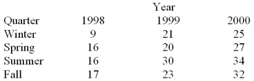
(Essay)
4.8/5 (39)
Filters
- Essay(0)
- Multiple Choice(0)
- Short Answer(0)
- True False(0)
- Matching(0)