Exam 16: Time Series Forecasting
Exam 1: An Introduction to Business Statistics54 Questions
Exam 2: Descriptive Statistics: Tabular and Graphical Methods90 Questions
Exam 3: Descriptive Statistics: Numerical Methods149 Questions
Exam 4: Probability135 Questions
Exam 5: Discrete Random Variables128 Questions
Exam 6: Continuous Random Variables150 Questions
Exam 7: Sampling and Sampling Distributions116 Questions
Exam 8: Confidence Intervals144 Questions
Exam 9: Hypothesis Testing148 Questions
Exam 10: Statistical Inferences Based on Two Samples132 Questions
Exam 11: Experimental Design and Analysis of Variance115 Questions
Exam 12: Chi-Square Tests96 Questions
Exam 13: Simple Linear Regression Analysis148 Questions
Exam 14: Multiple Regression122 Questions
Exam 15: Model Building and Model Diagnostics102 Questions
Exam 16: Time Series Forecasting150 Questions
Exam 17: Process Improvement Using Control Charts122 Questions
Exam 18: Nonparametric Methods97 Questions
Exam 19: Decision Theory90 Questions
Select questions type
The following data on prices and quantities for the years 1995 and 2000 are given for three products. 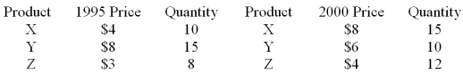 Calculate the aggregate price index.
(Essay)
4.9/5  (36)
(36)
Suppose that the unadjusted seasonal factor for the month of April is 1.10.The sum of the 12 months' unadjusted seasonal factor values is 12.18.The normalized (adjusted)seasonal factor value for April is
(Multiple Choice)
4.7/5 (35)
When a forecaster uses the ______________ method she or he assumes that the time series components are changing slowly over time.
(Multiple Choice)
4.9/5 (39)
Simple exponential smoothing is an appropriate method for prediction purposes when there is a significant trend present in a time series data.
(True/False)
4.9/5 (35)
The _______ component of time series reflects the long-run decline or growth in a time series.
(Multiple Choice)
4.8/5 (31)
Consider the quarterly production data (in thousands of units)for the XYZ manufacturing company below. 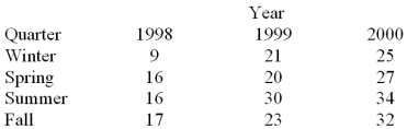 Calculate the average seasonal factor for each quarter
  .
Centered moving average values and their respective periods are given below.
.
Centered moving average values and their respective periods are given below. 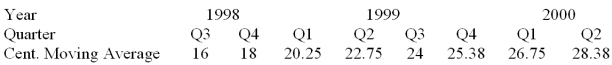
(Essay)
4.8/5 (39)
Assume that the current date is February 1,2003.The linear regression model was applied to a monthly time series data based on the last 24 months' sales.(from January 2000 through December 2002).The following partial computer output summarizes the results. 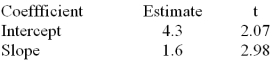 Determine the predicted sales for this month.
(Multiple Choice)
4.8/5 (37)
Consider the following set of quarterly sales data given in thousands of dollars. 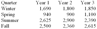 The following dummy variable model that incorporates a linear trend and constant seasonal variation was used: y (t)= B0 + B1t + BQ1(Q1)+ BQ2(Q2)+ BQ3(Q3)+ Et
In this model there are 3 binary seasonal variables (Q1,Q2,and Q3).
Where
Qi is a binary (0,1)variable defined as:
Qi = 1,if the time series data is associated with quarter i;
Qi = 0,if the time series data is not associated with quarter i.
The results associated with this data and model are given in the following MINITAB computer output.
The regression equation is
Sales = 2442 + 6.2 Time - 693 Q1 - 1499 Q2 + 153 Q3
The following dummy variable model that incorporates a linear trend and constant seasonal variation was used: y (t)= B0 + B1t + BQ1(Q1)+ BQ2(Q2)+ BQ3(Q3)+ Et
In this model there are 3 binary seasonal variables (Q1,Q2,and Q3).
Where
Qi is a binary (0,1)variable defined as:
Qi = 1,if the time series data is associated with quarter i;
Qi = 0,if the time series data is not associated with quarter i.
The results associated with this data and model are given in the following MINITAB computer output.
The regression equation is
Sales = 2442 + 6.2 Time - 693 Q1 - 1499 Q2 + 153 Q3  At = .05,test the significance of the model.
(Essay)
4.8/5 (40)
The price and quantity of several food items are listed below for the years 1990 and 2000. 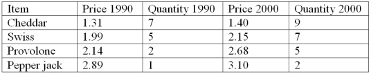 Compute the Paasche index using 1990 as the base year.
(Essay)
4.9/5 (36)
Use the following information for the three grains. 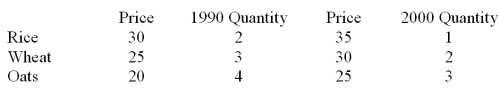 Calculate the aggregate price index.
(Essay)
5.0/5 (37)
Consider the following set of quarterly sales data given in thousands of dollars. 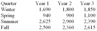 The following dummy variable model that incorporates a linear trend and constant seasonal variation was used: y (t)= B0 + B1t + BQ1(Q1)+ BQ2(Q2)+ BQ3(Q3)+ Et
In this model there are 3 binary seasonal variables (Q1,Q2,and Q3).
Where
Qi is a binary (0,1)variable defined as:
Qi = 1,if the time series data is associated with quarter i;
Qi = 0,if the time series data is not associated with quarter i.
The results associated with this data and model are given in the following MINITAB computer output.
The regression equation is
Sales = 2442 + 6.2 Time - 693 Q1 - 1499 Q2 + 153 Q3
The following dummy variable model that incorporates a linear trend and constant seasonal variation was used: y (t)= B0 + B1t + BQ1(Q1)+ BQ2(Q2)+ BQ3(Q3)+ Et
In this model there are 3 binary seasonal variables (Q1,Q2,and Q3).
Where
Qi is a binary (0,1)variable defined as:
Qi = 1,if the time series data is associated with quarter i;
Qi = 0,if the time series data is not associated with quarter i.
The results associated with this data and model are given in the following MINITAB computer output.
The regression equation is
Sales = 2442 + 6.2 Time - 693 Q1 - 1499 Q2 + 153 Q3 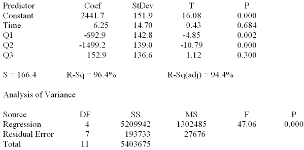 Provide a managerial interpretation of the regression coefficient for the variable "time."
(Essay)
4.8/5 (36)
Given the following data 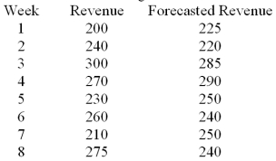 Compute the total error (sum of the error terms).
(Multiple Choice)
4.9/5 (37)
While a simple index is calculated by using the values of one time series,an aggregate index is computed based on the accumulated values of more than one time series.
(True/False)
4.7/5 (36)
Paasche index more accurately provides a year-to-year comparison of the annual cost of selected products in the market-basket than Laspeyres index.
(True/False)
4.8/5 (43)
The purpose behind moving averages and centered moving averages is to eliminate _________________.
(Multiple Choice)
4.9/5 (35)
The ________ component of a time series measures the fluctuations in a time series due to economic conditions of prosperity and recession with a duration of approximately 2 years or longer.
(Multiple Choice)
4.8/5 (36)
The linear regression trend model was applied to a time series of sales data based on the last 16 months of sales.The following partial computer output was obtained: 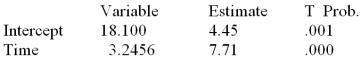 Test the significance of the time term at = .05.State the critical t value and make your decision using a two-sided alternative.
(Essay)
4.7/5 (39)
Based on the quarterly production data (in thousands of units)for the XYZ manufacturing company,the average seasonal factor  is .986 for winter,.915 for spring,1.125 for summer and .925 for fall.Determine the normalized (adjusted)seasonal factors for each quarter.
(Essay)
4.7/5 (42)
Assume that the current date is February 1,2003.The linear regression model was applied to a monthly time series data based on the last 24 months' sales.(from January 2000 through December 2002).The following partial computer output summarizes the results. 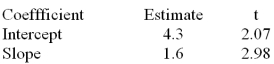 At a significance level of .05,what is the value of the rejection point in testing the slope for significance?
(Multiple Choice)
4.8/5 (39)
Filters
- Essay(0)
- Multiple Choice(0)
- Short Answer(0)
- True False(0)
- Matching(0)