Exam 16: Regression Models for Nonlinear Relationships
Exam 1: Statistics and Data68 Questions
Exam 2: Tabular and Graphical Methods99 Questions
Exam 3: Numerical Descriptive Measures123 Questions
Exam 4: Basic Probability Concepts107 Questions
Exam 5: Discrete Probability Distributions118 Questions
Exam 6: Continuous Probability Distributions114 Questions
Exam 7: Sampling and Sampling Distributions110 Questions
Exam 8: Interval Estimation111 Questions
Exam 9: Hypothesis Testing111 Questions
Exam 10: Statistical Inference Concerning Two Populations104 Questions
Exam 11: Statistical Inference Concerning Variance96 Questions
Exam 12: Chi-Square Tests100 Questions
Exam 13: Analysis of Variance89 Questions
Exam 14: Regression Analysis116 Questions
Exam 15: Inference With Regression Models117 Questions
Exam 16: Regression Models for Nonlinear Relationships95 Questions
Exam 17: Regression Models With Dummy Variables117 Questions
Exam 18: Time Series and Forecasting103 Questions
Exam 19: Returns, Index Numbers and Inflation98 Questions
Exam 20: Nonparametric Tests99 Questions
Select questions type
Exhibit 16.6.Thirty employed single individuals were randomly selected to examine the relationship between their age (Age)and their credit card debt (Debt)expressed as a percentage of their annual income.Three polynomial models were applied and the following table summarizes Excel's regression results.  Refer to Exhibit 16.6.What is the regression equation that provides the best fit?
(Essay)
4.8/5  (43)
(43)
For the exponential model ln(y)= β0 + β1x + ε,if x increases by 1 unit,then E(y)changes by approximately
(Multiple Choice)
4.9/5 (36)
Exhibit 16-4.The following data shows the cooling temperatures of a freshly brewed cup of coffee after it is poured from the brewing pot into a serving cup.The brewing pot temperature is approximately 180º F;see http://mathbits.com/mathbits/tisection/statistics2/exponential.htm 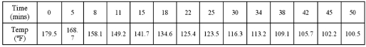 For the assumed exponential model ln(Temp)= β0 + β1Time + ε,the following Excel regression partial output is available.
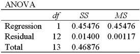
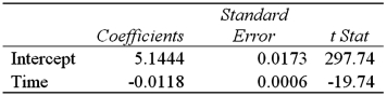 Refer to Exhibit 16-4.What is the predicted coffee temperature in half an hour after the brewing?
(Multiple Choice)
4.7/5 (38)
Exhibit 16-4.The following data shows the cooling temperatures of a freshly brewed cup of coffee after it is poured from the brewing pot into a serving cup.The brewing pot temperature is approximately 180º F;see http://mathbits.com/mathbits/tisection/statistics2/exponential.htm  For the assumed exponential model ln(Temp)= β0 + β1Time + ε,the following Excel regression partial output is available.
 Refer to Exhibit 16-4.What is the sample correlation coefficient between ln(Temp)and Time?
(Multiple Choice)
4.9/5 (33)
Exhibit 16.6.Thirty employed single individuals were randomly selected to examine the relationship between their age (Age)and their credit card debt (Debt)expressed as a percentage of their annual income.Three polynomial models were applied and the following table summarizes Excel's regression results. 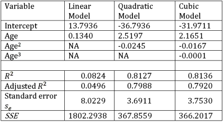 Refer to Exhibit 16.6.For the cubic model,Debt = β0 + β1Age + β2Age2+ β3Age3 + ε,the following Excel partial output is available.What is the conclusion when testing the individual significance of Age3?
(Essay)
4.9/5 (37)
Exhibit 16.6.Thirty employed single individuals were randomly selected to examine the relationship between their age (Age)and their credit card debt (Debt)expressed as a percentage of their annual income.Three polynomial models were applied and the following table summarizes Excel's regression results.  Refer to Exhibit 16.6.If you impose the restrictions β2 = β3 = 0 on the model Debt = β0 + β1Age + β2Age2+ β3Age3 + ε,what will be the sum of the squared errors (SSER)computed for the restricted model?
(Essay)
4.8/5 (42)
For the exponential model ln(y)= β0 + β1x + ε,β1 × 100% is the approximate percentage change in E(y)when x increases by one percent.
(True/False)
4.9/5 (44)
Exhibit 16.5.The following data shows the demand for an airline ticket dependent on the price of this ticket. 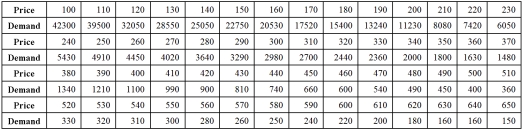 For the assumed cubic and log-log regression models,Demand = β0 + β1Price + β2Price2 + β3Price3 + ε and ln(Demand)= β0 + β1ln(Price)+ ε,the following regression results are available:
 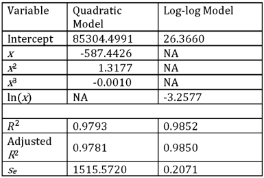 Refer to Exhibit 16.5.Using the log-log model,what is the predicted demand when the price is $200?
(Multiple Choice)
4.8/5 (33)
Exhibit 16-7.It is believed that the sales volume of one liter Pepsi bottles depends on the price of the bottle and the price of one liter bottle of Coca Cola.The following data has been collected for a certain sales region.  Using Excel's regression,the linear model PepsiSales = β0 + β1PepsiPrice + β2ColaPrice + ε and the log-log model ln(PepsiSales)= β0 + β1ln(PepsiPrice)+ β2ln(ColaPrice)+ ε have been estimated as follows:
 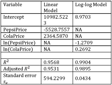 Refer to Exhibit 16.7.What is the percentage of variations in ln(PepsiSales)explained by the estimated log-log model?
(Short Answer)
4.9/5 (42)
For the log-log model ln(y)= β0 + β1ln(x)+ ε,the predicted value of y is computed by:
(Multiple Choice)
4.8/5 (26)
Exhibit 16.2.Typically,the sales volume declines with an increase of a product price.It has been observed,however,that for some luxury goods the sales volume may increase when the price increases.The following Excel output illustrates this rather unusual relationship. 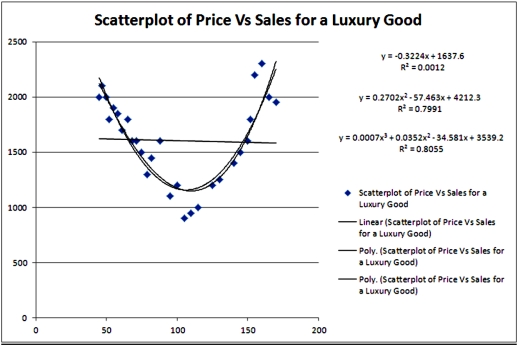 Refer to Exhibit 16.2.For which two prices are the sales predicted by the quadratic equation are 1700 units?
(Multiple Choice)
5.0/5 (40)
Exhibit 16.5.The following data shows the demand for an airline ticket dependent on the price of this ticket.  For the assumed cubic and log-log regression models,Demand = β0 + β1Price + β2Price2 + β3Price3 + ε and ln(Demand)= β0 + β1ln(Price)+ ε,the following regression results are available:
  Refer to Exhibit 16.5.Assuming that the sample correlation coefficient between Demand and
  is 0.956,what is the percentage of variations in Demand explained by the log-log regression equation?
(Multiple Choice)
4.9/5 (35)
The logarithmic and log-log models,y = β0 + β1ln(x)+ ε and ln(y)= β0 + β1ln(x)+ ε,were used to fit given data on y and x,and the following table summarizes the regression results.Which of the two models provides a better fit? 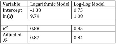
(Multiple Choice)
4.9/5 (31)
Exhibit 16.6.Thirty employed single individuals were randomly selected to examine the relationship between their age (Age)and their credit card debt (Debt)expressed as a percentage of their annual income.Three polynomial models were applied and the following table summarizes Excel's regression results.  Refer to Exhibit 16.6.Using the quadratic regression equation,find the age of an employed single person with the highest predicted percentage debt.
(Short Answer)
4.8/5 (40)
The fit of the models y = β0 + β1x + ε and ln(y)= β0 + β1x + ε can be compared using the coefficients R2 found in the two corresponding Excel's regression outputs.
(True/False)
4.8/5 (26)
Exhibit 16-7.It is believed that the sales volume of one liter Pepsi bottles depends on the price of the bottle and the price of one liter bottle of Coca Cola.The following data has been collected for a certain sales region. 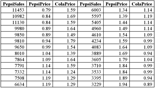 Using Excel's regression,the linear model PepsiSales = β0 + β1PepsiPrice + β2ColaPrice + ε and the log-log model ln(PepsiSales)= β0 + β1ln(PepsiPrice)+ β2ln(ColaPrice)+ ε have been estimated as follows:
  Refer to Exhibit 16.7.What is the estimated linear regression model?
(Essay)
4.7/5 (30)
Which of the regression models is most likely to provide the best fit for the data represented by the following scatterplot? 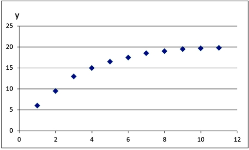
(Multiple Choice)
4.9/5 (37)
Exhibit 16-1.The following Excel scatterplot with the fitted quadratic regression equation illustrates the observed relationship between productivity and the number of hired workers. 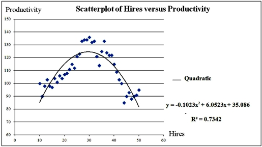 Refer to Exhibit 16.1.Predict the productivity when 32 workers are hired.
(Multiple Choice)
4.7/5 (33)
For the quadratic regression equation  ,the optimum (maximum or minimum)value of
  is:
is:
(Multiple Choice)
4.7/5 (31)
Filters
- Essay(0)
- Multiple Choice(0)
- Short Answer(0)
- True False(0)
- Matching(0)