Exam 16: Regression Models for Nonlinear Relationships
Exam 1: Statistics and Data68 Questions
Exam 2: Tabular and Graphical Methods99 Questions
Exam 3: Numerical Descriptive Measures123 Questions
Exam 4: Basic Probability Concepts107 Questions
Exam 5: Discrete Probability Distributions118 Questions
Exam 6: Continuous Probability Distributions114 Questions
Exam 7: Sampling and Sampling Distributions110 Questions
Exam 8: Interval Estimation111 Questions
Exam 9: Hypothesis Testing111 Questions
Exam 10: Statistical Inference Concerning Two Populations104 Questions
Exam 11: Statistical Inference Concerning Variance96 Questions
Exam 12: Chi-Square Tests100 Questions
Exam 13: Analysis of Variance89 Questions
Exam 14: Regression Analysis116 Questions
Exam 15: Inference With Regression Models117 Questions
Exam 16: Regression Models for Nonlinear Relationships95 Questions
Exam 17: Regression Models With Dummy Variables117 Questions
Exam 18: Time Series and Forecasting103 Questions
Exam 19: Returns, Index Numbers and Inflation98 Questions
Exam 20: Nonparametric Tests99 Questions
Select questions type
The coefficient of determination R2 cannot be used to compare the linear and quadratic models,because:
(Multiple Choice)
4.8/5  (28)
(28)
Exhibit 16-7.It is believed that the sales volume of one liter Pepsi bottles depends on the price of the bottle and the price of one liter bottle of Coca Cola.The following data has been collected for a certain sales region. 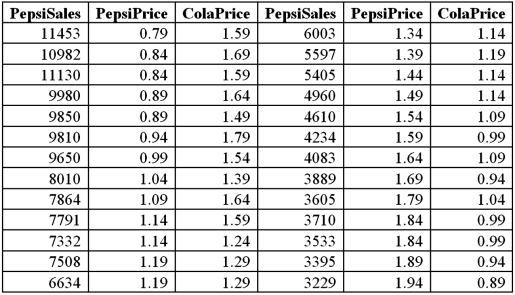 Using Excel's regression,the linear model PepsiSales = β0 + β1PepsiPrice + β2ColaPrice + ε and the log-log model ln(PepsiSales)= β0 + β1ln(PepsiPrice)+ β2ln(ColaPrice)+ ε have been estimated as follows:
  Refer to Exhibit 16.7.For the estimated log-log model,interpret the estimated coefficient of ln(PepsiPrice).
(Essay)
4.8/5 (36)
Exhibit 16-4.The following data shows the cooling temperatures of a freshly brewed cup of coffee after it is poured from the brewing pot into a serving cup.The brewing pot temperature is approximately 180º F;see http://mathbits.com/mathbits/tisection/statistics2/exponential.htm  For the assumed exponential model ln(Temp)= β0 + β1Time + ε,the following Excel regression partial output is available.
 Refer to Exhibit 16-4.How many minutes must elapse after the brewing in order to cool the coffee to 158 oF?
(Multiple Choice)
4.8/5 (28)
Exhibit 16.2.Typically,the sales volume declines with an increase of a product price.It has been observed,however,that for some luxury goods the sales volume may increase when the price increases.The following Excel output illustrates this rather unusual relationship. 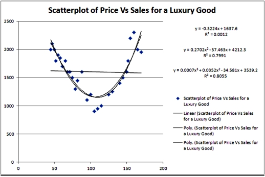 Refer to Exhibit 16.2.For the considered range of the price,the relationship between Price and Sales should be described by a:
(Multiple Choice)
4.8/5 (37)
Exhibit 16-7.It is believed that the sales volume of one liter Pepsi bottles depends on the price of the bottle and the price of one liter bottle of Coca Cola.The following data has been collected for a certain sales region.  Using Excel's regression,the linear model PepsiSales = β0 + β1PepsiPrice + β2ColaPrice + ε and the log-log model ln(PepsiSales)= β0 + β1ln(PepsiPrice)+ β2ln(ColaPrice)+ ε have been estimated as follows:
  Refer to Exhibit 16.7.For the estimated log-log model,interpret the estimated coefficient of ln(ColaPrice).
(Essay)
4.9/5 (36)
Exhibit 16.5.The following data shows the demand for an airline ticket dependent on the price of this ticket. 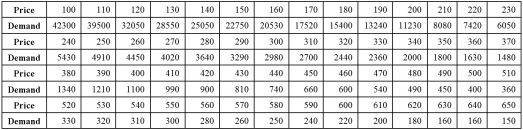 For the assumed cubic and log-log regression models,Demand = β0 + β1Price + β2Price2 + β3Price3 + ε and ln(Demand)= β0 + β1ln(Price)+ ε,the following regression results are available:
 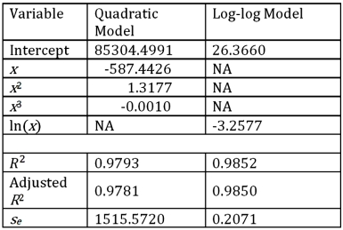 Refer to Exhibit 16.5.Using the cubic model,what is the predicted demand when the price is $200?
(Multiple Choice)
4.8/5 (44)
Exhibit 16.5.The following data shows the demand for an airline ticket dependent on the price of this ticket.  For the assumed cubic and log-log regression models,Demand = β0 + β1Price + β2Price2 + β3Price3 + ε and ln(Demand)= β0 + β1ln(Price)+ ε,the following regression results are available:
  Refer to Exhibit 16.5.Assuming that the sample correlation coefficient between Demand and
  is 0.956,what is the predicted demand for a price of $250 found by the model with better fit?
(Multiple Choice)
4.8/5 (31)
Exhibit 16-7.It is believed that the sales volume of one liter Pepsi bottles depends on the price of the bottle and the price of one liter bottle of Coca Cola.The following data has been collected for a certain sales region.  Using Excel's regression,the linear model PepsiSales = β0 + β1PepsiPrice + β2ColaPrice + ε and the log-log model ln(PepsiSales)= β0 + β1ln(PepsiPrice)+ β2ln(ColaPrice)+ ε have been estimated as follows:
  Refer to Exhibit 16.7.What is the percentage of variations in the sales of Pepsi explained by the estimated linear model?
(Short Answer)
4.8/5 (49)
Exhibit 16-7.It is believed that the sales volume of one liter Pepsi bottles depends on the price of the bottle and the price of one liter bottle of Coca Cola.The following data has been collected for a certain sales region.  Using Excel's regression,the linear model PepsiSales = β0 + β1PepsiPrice + β2ColaPrice + ε and the log-log model ln(PepsiSales)= β0 + β1ln(PepsiPrice)+ β2ln(ColaPrice)+ ε have been estimated as follows:
 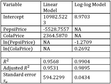 Refer to Exhibit 16.7.For the estimated linear model,when the price of Cola is held constant what is the predicted change in the Pepsi sales if the price of Pepsi increases by 10 cents?
(Essay)
4.8/5 (35)
Exhibit 16-1.The following Excel scatterplot with the fitted quadratic regression equation illustrates the observed relationship between productivity and the number of hired workers. 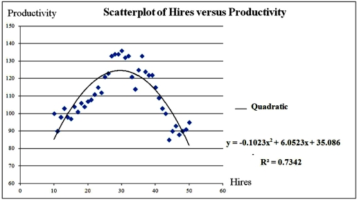 Refer to Exhibit 16.1.Assuming that the number of hired workers must be integer,how many workers should be hired in order to achieve the highest productivity?
(Multiple Choice)
4.9/5 (35)
Exhibit 16-7.It is believed that the sales volume of one liter Pepsi bottles depends on the price of the bottle and the price of one liter bottle of Coca Cola.The following data has been collected for a certain sales region.  Using Excel's regression,the linear model PepsiSales = β0 + β1PepsiPrice + β2ColaPrice + ε and the log-log model ln(PepsiSales)= β0 + β1ln(PepsiPrice)+ β2ln(ColaPrice)+ ε have been estimated as follows:
  Refer to Exhibit 16.7.Discuss the choice between the linear model and the log-log model.
(Essay)
5.0/5 (29)
Exhibit 16.5.The following data shows the demand for an airline ticket dependent on the price of this ticket.  For the assumed cubic and log-log regression models,Demand = β0 + β1Price + β2Price2 + β3Price3 + ε and ln(Demand)= β0 + β1ln(Price)+ ε,the following regression results are available:
  Refer to Exhibit 16.5.What is the percentage of variations in ln(Demand)explained by the log-log regression equation?
(Multiple Choice)
4.7/5 (36)
A quadratic regression model is a special type of a polynomial regression model.
(True/False)
4.9/5 (36)
For the quadratic equation 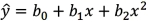 ,which of the following expressions must be zero in order to minimize or maximize the predicted y?
(Multiple Choice)
4.9/5 (33)
Exhibit 16-4.The following data shows the cooling temperatures of a freshly brewed cup of coffee after it is poured from the brewing pot into a serving cup.The brewing pot temperature is approximately 180º F;see http://mathbits.com/mathbits/tisection/statistics2/exponential.htm 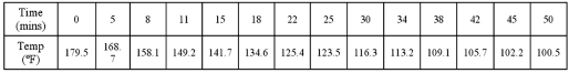 For the assumed exponential model ln(Temp)= β0 + β1Time + ε,the following Excel regression partial output is available.
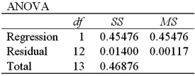
 Refer to Exhibit 16-4.What is the regression equation for making predictions concerning the coffee temperature?
(Multiple Choice)
4.9/5 (36)
Exhibit 16.2.Typically,the sales volume declines with an increase of a product price.It has been observed,however,that for some luxury goods the sales volume may increase when the price increases.The following Excel output illustrates this rather unusual relationship.  Refer to Exhibit 16.2.What can be said about the linear relationship between Price and Sales?
(Multiple Choice)
4.7/5 (38)
When the data is available on x and y,it is easy to estimate a polynomial regression model.
(True/False)
4.8/5 (40)
The fit of the models y = β0 + β1x + β2x2 + ε and y = β0 + β1ln(x)+ ε can be compared using the coefficient of determination R2.
(True/False)
4.8/5 (27)
The cubic regression model,y = β0 + β1x + β2x2+ β3x3 + ε,is used when we assume that the relationship between x and y should be captured by a function that has either minimum or maximum,but not both.
(True/False)
4.9/5 (32)
Exhibit 16-4.The following data shows the cooling temperatures of a freshly brewed cup of coffee after it is poured from the brewing pot into a serving cup.The brewing pot temperature is approximately 180º F;see http://mathbits.com/mathbits/tisection/statistics2/exponential.htm  For the assumed exponential model ln(Temp)= β0 + β1Time + ε,the following Excel regression partial output is available.
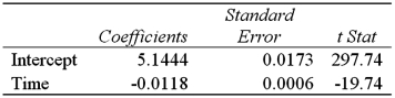 Refer to Exhibit 16-4.What is the standard error of the estimate?
(Multiple Choice)
4.8/5 (32)
Filters
- Essay(0)
- Multiple Choice(0)
- Short Answer(0)
- True False(0)
- Matching(0)