Exam 16: Regression Models for Nonlinear Relationships
Exam 1: Statistics and Data68 Questions
Exam 2: Tabular and Graphical Methods99 Questions
Exam 3: Numerical Descriptive Measures123 Questions
Exam 4: Basic Probability Concepts107 Questions
Exam 5: Discrete Probability Distributions118 Questions
Exam 6: Continuous Probability Distributions114 Questions
Exam 7: Sampling and Sampling Distributions110 Questions
Exam 8: Interval Estimation111 Questions
Exam 9: Hypothesis Testing111 Questions
Exam 10: Statistical Inference Concerning Two Populations104 Questions
Exam 11: Statistical Inference Concerning Variance96 Questions
Exam 12: Chi-Square Tests100 Questions
Exam 13: Analysis of Variance89 Questions
Exam 14: Regression Analysis116 Questions
Exam 15: Inference With Regression Models117 Questions
Exam 16: Regression Models for Nonlinear Relationships95 Questions
Exam 17: Regression Models With Dummy Variables117 Questions
Exam 18: Time Series and Forecasting103 Questions
Exam 19: Returns, Index Numbers and Inflation98 Questions
Exam 20: Nonparametric Tests99 Questions
Select questions type
For the model ln(y)= β0 + β1ln(x)+ ε with 0 < β1 < 1,if x increases than E(y)increases but at a slower rate.
(True/False)
4.8/5  (43)
(43)
In the model ln(y)= β0 + β1ln(x)+ ε,the coefficient β1 is the approximate:
(Multiple Choice)
4.8/5 (36)
Exhibit 16-1.The following Excel scatterplot with the fitted quadratic regression equation illustrates the observed relationship between productivity and the number of hired workers. 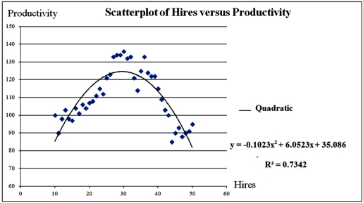 Refer to Exhibit 16.1.What is the percentage of variations in the productivity explained by the number of hired workers?
(Multiple Choice)
4.7/5 (34)
How many coefficients have to be estimated in the quadratic regression modely = β0 + β1x + β2x2 + ε?
(Multiple Choice)
4.8/5 (26)
Exhibit 16.2.Typically,the sales volume declines with an increase of a product price.It has been observed,however,that for some luxury goods the sales volume may increase when the price increases.The following Excel output illustrates this rather unusual relationship. 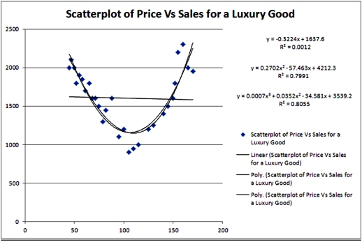 Refer to Exhibit 16.2.Using the quadratic equation,predict the sales if the luxury good is priced at $100.
(Multiple Choice)
4.8/5 (39)
The curve representing the regression equation 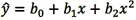 has a U-shape if b2 > 0.
(True/False)
4.8/5 (36)
Exhibit 16.2.Typically,the sales volume declines with an increase of a product price.It has been observed,however,that for some luxury goods the sales volume may increase when the price increases.The following Excel output illustrates this rather unusual relationship.  Refer to Exhibit 16.2.For which price do sales predicted by the quadratic equation reach their minimum?
(Multiple Choice)
4.7/5 (37)
Exhibit 16-4.The following data shows the cooling temperatures of a freshly brewed cup of coffee after it is poured from the brewing pot into a serving cup.The brewing pot temperature is approximately 180º F;see http://mathbits.com/mathbits/tisection/statistics2/exponential.htm 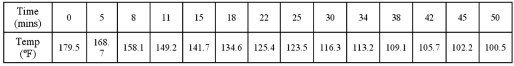 For the assumed exponential model ln(Temp)= β0 + β1Time + ε,the following Excel regression partial output is available.
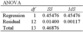
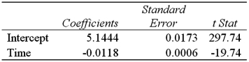 Refer to Exhibit 16-4.During one minute,the predicted temperature decreases by approximately
(Multiple Choice)
4.8/5 (46)
The fit of the regression equations 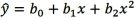 and
and 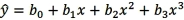 can be compared using the coefficient of determination R2.
(True/False)
4.8/5 (37)
Exhibit 16.2.Typically,the sales volume declines with an increase of a product price.It has been observed,however,that for some luxury goods the sales volume may increase when the price increases.The following Excel output illustrates this rather unusual relationship.  Refer to Exhibit 16.2.Which of the following models is most likely to be chosen in order to describe the relationship between Price and Sales?
(Multiple Choice)
4.8/5 (36)
Exhibit 16.6.Thirty employed single individuals were randomly selected to examine the relationship between their age (Age)and their credit card debt (Debt)expressed as a percentage of their annual income.Three polynomial models were applied and the following table summarizes Excel's regression results.  Refer to Exhibit 16.6.Suppose the restriction β3 = 0 is imposed on the cubic model Debt = β0 + β1Age + β2Age2+ β3Age3 + ε.What regression equation is obtained under this restriction?
(Essay)
5.0/5 (36)
The linear and logarithmic models,y = β0 + β1x + ε and y = β0 + β1ln(x)+ ε,were used to fit given data on y and x,and the following table summarizes the regression results.Which of the two models provides a better fit? 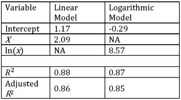
(Multiple Choice)
4.8/5 (37)
For the logarithmic model y = β0 + β1ln(x)+ ε,β1/100 is the approximate change in E(y)when x increases by one percent.
(True/False)
4.7/5 (30)
What does a positive value for price elasticity indicate if y represents the quantity demanded of a particular good and x is its unit price in a log-log regression model?
(Multiple Choice)
5.0/5 (35)
Exhibit 16.6.Thirty employed single individuals were randomly selected to examine the relationship between their age (Age)and their credit card debt (Debt)expressed as a percentage of their annual income.Three polynomial models were applied and the following table summarizes Excel's regression results. 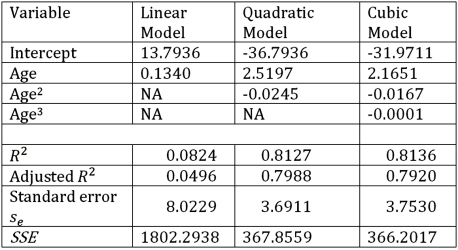 Refer to Exhibit 16.6.What is the predicted percentage debt of a 45 year old employed single person determined by the model with the best fit?
(Short Answer)
4.9/5 (31)
Filters
- Essay(0)
- Multiple Choice(0)
- Short Answer(0)
- True False(0)
- Matching(0)