Exam 15: Inference With Regression Models
Exam 1: Statistics and Data68 Questions
Exam 2: Tabular and Graphical Methods99 Questions
Exam 3: Numerical Descriptive Measures123 Questions
Exam 4: Basic Probability Concepts107 Questions
Exam 5: Discrete Probability Distributions118 Questions
Exam 6: Continuous Probability Distributions114 Questions
Exam 7: Sampling and Sampling Distributions110 Questions
Exam 8: Interval Estimation111 Questions
Exam 9: Hypothesis Testing111 Questions
Exam 10: Statistical Inference Concerning Two Populations104 Questions
Exam 11: Statistical Inference Concerning Variance96 Questions
Exam 12: Chi-Square Tests100 Questions
Exam 13: Analysis of Variance89 Questions
Exam 14: Regression Analysis116 Questions
Exam 15: Inference With Regression Models117 Questions
Exam 16: Regression Models for Nonlinear Relationships95 Questions
Exam 17: Regression Models With Dummy Variables117 Questions
Exam 18: Time Series and Forecasting103 Questions
Exam 19: Returns, Index Numbers and Inflation98 Questions
Exam 20: Nonparametric Tests99 Questions
Select questions type
Consider the following simple linear regression model: 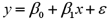 .When determining whether there is a positive linear relationship between x and y,the alternative hypothesis takes the form
(Multiple Choice)
4.9/5  (31)
(31)
If the variance of the error term is not the same for all observations,we
(Multiple Choice)
4.8/5 (40)
Given the following portion of regression results,what is the value of the  test statistic?
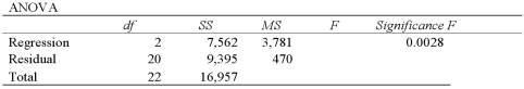
(Multiple Choice)
4.9/5 (40)
Exhibit 15-6.Tiffany & Co.has been the world's premier jeweler since 1837.The performance of Tiffany's stock is likely to be strongly influenced by the economy.Monthly data for Tiffany's risk-adjusted return and the risk-adjusted market return are collected for a five-year period (n = 60).The accompanying table shows the regression results when estimating the CAPM model for Tiffany's return. 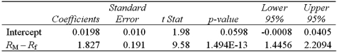 Refer to Exhibit 15-6.To determine whether abnormal returns exist,which of the following competing hypotheses do you set up?
(Multiple Choice)
4.8/5 (39)
Exhibit 15-2.A sports analyst wants to exam the factors that may influence a tennis player's chances of winning.Over four tournaments,he collects data on 30 tennis players and estimates the following model:  , where Win is the proportion of winning,Double Faults is the percentage of double faults made,and Aces is the number of Aces.A portion of the regression results are shown in the accompanying table.
  Refer to Exhibit 15-2.When testing whether the explanatory variables are jointly significant at the 5% level,he
(Multiple Choice)
4.9/5 (36)
Exhibit 15-1.An marketing analyst wants to examine the relationship between sales (in $1,000s)and advertising (in $100s)for firms in the food and beverage industry and so collects monthly data for 25 firms.He estimates the model  .The following table shows a portion of the regression results.
  Refer to Exhibit 15-1.When testing whether Advertising is significant at the 10% significance level,the conclusion is to
(Multiple Choice)
4.8/5 (32)
Exhibit 15-2.A sports analyst wants to exam the factors that may influence a tennis player's chances of winning.Over four tournaments,he collects data on 30 tennis players and estimates the following model:  , where Win is the proportion of winning,Double Faults is the percentage of double faults made,and Aces is the number of Aces.A portion of the regression results are shown in the accompanying table.
 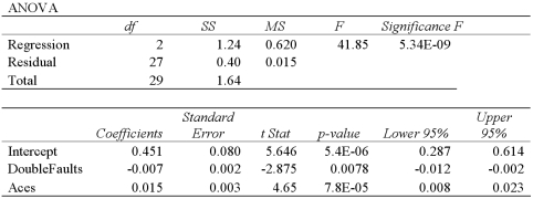 Refer to Exhibit 15-2.Is the relationship between Win and Aces significant at the 5 percent level?
(Multiple Choice)
4.9/5 (37)
Exhibit 15-8.A real estate analyst believes that the three main factors that influence an apartment's rent in a college town are the number of bedrooms,the number of bathrooms,and the apartment's square footage.For 40 apartments,she collects data on the rent (y,in $),the number of bedrooms (x1),the number of bathrooms (x2),and its square footage (x3).She estimates the following model:  .The following table shows a portion of the regression results.
 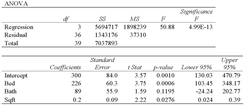 Refer to Exhibit 15-8.When testing whether Bed is significant at the 5% level,she
(Multiple Choice)
4.8/5 (40)
Exhibit 15-5.The accompanying table shows the regression results when estimating 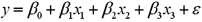 .
. 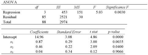 Refer to Exhibit 15-5.When testing whether or not x1 and x2 have the same influence on y,the null hypothesis is
(Multiple Choice)
4.8/5 (36)
Exhibit 15-2.A sports analyst wants to exam the factors that may influence a tennis player's chances of winning.Over four tournaments,he collects data on 30 tennis players and estimates the following model: ![Exhibit 15-2.A sports analyst wants to exam the factors that may influence a tennis player's chances of winning.Over four tournaments,he collects data on 30 tennis players and estimates the following model: , where Win is the proportion of winning,Double Faults is the percentage of double faults made,and Aces is the number of Aces.A portion of the regression results are shown in the accompanying table. Refer to Exhibit 15-2.Excel shows that the 95% confidence interval for β<sub>1</sub> is [-0.12,-0.002].When determining whether or not Double Faults is significant at the 5% significance level,he](https://storage.examlex.com/TB2339/11eaa4ae_7a81_e867_9180_eb104780023c_TB2339_00.jpg) , where Win is the proportion of winning,Double Faults is the percentage of double faults made,and Aces is the number of Aces.A portion of the regression results are shown in the accompanying table.
, where Win is the proportion of winning,Double Faults is the percentage of double faults made,and Aces is the number of Aces.A portion of the regression results are shown in the accompanying table. ![Exhibit 15-2.A sports analyst wants to exam the factors that may influence a tennis player's chances of winning.Over four tournaments,he collects data on 30 tennis players and estimates the following model: , where Win is the proportion of winning,Double Faults is the percentage of double faults made,and Aces is the number of Aces.A portion of the regression results are shown in the accompanying table. Refer to Exhibit 15-2.Excel shows that the 95% confidence interval for β<sub>1</sub> is [-0.12,-0.002].When determining whether or not Double Faults is significant at the 5% significance level,he](https://storage.examlex.com/TB2339/11eaa4ae_7a82_0f78_9180_45b91d73b619_TB2339_00.jpg) Refer to Exhibit 15-2.Excel shows that the 95% confidence interval for β1 is [-0.12,-0.002].When determining whether or not Double Faults is significant at the 5% significance level,he
Refer to Exhibit 15-2.Excel shows that the 95% confidence interval for β1 is [-0.12,-0.002].When determining whether or not Double Faults is significant at the 5% significance level,he
(Multiple Choice)
4.9/5 (36)
In a simple linear regression based on 30 observations,the following information is provided: 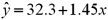 and
and  .Also,
  evaluated at
  is 1.3.
A)Construct a 95% confidence interval for E(y)if x = 20.
B)Construct a 95% prediction interval for y if x = 20.
is 1.3.
A)Construct a 95% confidence interval for E(y)if x = 20.
B)Construct a 95% prediction interval for y if x = 20.
(Essay)
4.8/5 (26)
When estimating a multiple regression model based on 30 observations,the following results were obtained.
(Essay)
4.9/5 (26)
For a given confidence level,the prediction interval is always wider than the confidence interval because
(Multiple Choice)
4.9/5 (41)
A simple linear regression, ,is estimated using time-series data over the last 10 years.The residuals e,and the time variable t are shown in the accompanying table.
  a.Graph the residuals e against time and look for any discernible pattern.
b.Which assumption is being violated? Discuss its consequences and suggest a possible remedy.
a.Graph the residuals e against time and look for any discernible pattern.
b.Which assumption is being violated? Discuss its consequences and suggest a possible remedy.
(Essay)
4.8/5 (32)
Exhibit 15-8.A real estate analyst believes that the three main factors that influence an apartment's rent in a college town are the number of bedrooms,the number of bathrooms,and the apartment's square footage.For 40 apartments,she collects data on the rent (y,in $),the number of bedrooms (x1),the number of bathrooms (x2),and its square footage (x3).She estimates the following model:  .The following table shows a portion of the regression results.
  Refer to Exhibit 15-8.Which of the following are the hypotheses to test if the explanatory variables Bath and Sqft are jointly significant in explaining Rent?
(Multiple Choice)
4.8/5 (36)
The accompanying table shows the regression results when estimating 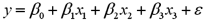 .At the 5% significance level,which explanatory variable(s)is(are)individually significant?
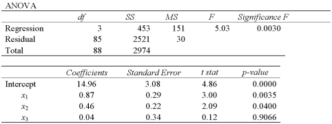
(Multiple Choice)
4.9/5 (32)
A sociologist estimates the following regression relating Poverty (y)to Education (x1):  In an attempt to improve the results,he adds two more explanatory variables: Median Income (x2,in $1,000s)and the Mortality Rate (x3,per 1,000 residents).The estimated regression equation is:
 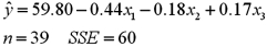 a.Formulate the hypotheses to determine whether Median Income and the Mortality Rate are jointly significant in explaining Poverty.
B)Calculate the value of the test statistic.
C)At the 5% significance level,find the approximate value of the critical value(s).
D)What is the conclusion to the test?
a.Formulate the hypotheses to determine whether Median Income and the Mortality Rate are jointly significant in explaining Poverty.
B)Calculate the value of the test statistic.
C)At the 5% significance level,find the approximate value of the critical value(s).
D)What is the conclusion to the test?
(Essay)
4.9/5 (29)
Filters
- Essay(0)
- Multiple Choice(0)
- Short Answer(0)
- True False(0)
- Matching(0)