Exam 9: Assessing Studies Based on Multiple Regression
Exam 1: Economic Questions and Data17 Questions
Exam 2: Review of Probability71 Questions
Exam 3: Review of Statistics63 Questions
Exam 4: Linear Regression With One Regressor65 Questions
Exam 5: Regression With a Single Regressor: Hypothesis Tests and Confidence Intervals59 Questions
Exam 6: Linear Regression With Multiple Regressors65 Questions
Exam 7: Hypothesis Tests and Confidence Intervals in Multiple Regression65 Questions
Exam 8: Nonlinear Regression Functions62 Questions
Exam 9: Assessing Studies Based on Multiple Regression65 Questions
Exam 10: Regression With Panel Data50 Questions
Exam 11: Regression With a Binary Dependent Variable50 Questions
Exam 12: Instrumental Variables Regression50 Questions
Exam 13: Experiments and Quasi-Experiments50 Questions
Exam 14: Introduction to Time Series Regression and Forecasting50 Questions
Exam 15: Estimation of Dynamic Causal Effects50 Questions
Exam 16: Additional Topics in Time Series Regression50 Questions
Exam 17: The Theory of Linear Regression With One Regressor49 Questions
Exam 18: The Theory of Multiple Regression50 Questions
Select questions type
Suppose that you have just read a review of the literature of the effect of beauty on earnings.You were initially surprised to find a mild effect of beauty even on teaching evaluations at colleges.Intrigued by this effect,you consider explanations as to why more attractive individuals receive higher salaries.One of the possibilities you consider is that beauty may be a marker of performance/productivity.As a result,you set out to test whether or not more attractive individuals receive higher grades (cumulative GPA)at college.You happen to have access to individuals at two highly selective liberal arts colleges nearby.One of these specializes in Economics and Government and incoming students have an average SAT of 2,100;the other is known for its engineering program and has an incoming SAT average of 2,200.Conducting a survey,where you offer students a small incentive to answer a few questions regarding their academic performance,and taking a picture of these individuals,you establish that there is no relationship between grades and beauty.Write a short essay using some of the concepts of internal and external validity to determine if these results are likely to apply to universities in general.
(Essay)
4.9/5  (36)
(36)
The true causal effect might not be the same in the population studied and the population of interest because
(Multiple Choice)
4.9/5 (45)
Your textbook has analyzed simultaneous equation systems in the case of two equations,
Yi = β0 + β1Xi + ui
Xi =  +
+  Yi + vi,
where the first equation might be the labor demand equation (with capital stock and technology being held constant),and the second the labor supply equation (X being the real wage,and the labor market clears).What if you had a a production function as the third equation
Zi =
Yi + vi,
where the first equation might be the labor demand equation (with capital stock and technology being held constant),and the second the labor supply equation (X being the real wage,and the labor market clears).What if you had a a production function as the third equation
Zi =  +
+  Yi + wi
where Z is output.If the error terms,u,v,and w,were pairwise uncorrelated,explain why there would be no simultaneous causality bias when estimating the production function using OLS.
Yi + wi
where Z is output.If the error terms,u,v,and w,were pairwise uncorrelated,explain why there would be no simultaneous causality bias when estimating the production function using OLS.
(Essay)
4.7/5 (36)
Your professor wants to measure the class's knowledge of econometrics twice during the semester,once in a midterm and once in a final.Assume that your performance,and that of your peers,on the day of your midterm exam only measure knowledge imperfectly and with an error, 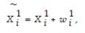 where
where  is your exam grade,X is underlying econometrics knowledge,and w is a random error with mean zero and variance
  .w may depend on whether you have a headache that day,whether or not the questions you had prepared for appeared on the exam,your mood,etc.A similar situation holds for the final,which is exam two:
  .What would happen if you ran a regression of grades received by students in the final on midterm grades?
(Essay)
4.8/5 (41)
In macroeconomics,you studied the equilibrium in the goods and money market under the assumption of prices being fixed in the very short run.The goods market equilibrium was described by the so-called IS equation
Ri = β0 - β1Yi + ui
where R represented the nominal interest rate and Y was real GDP.β0 contained variables determined outside the system,such as government expenditures,taxes,and inflationary expectations.
The money market equilibrium was given by the so-called LM equation
Ri =  +
+  Yi + vi
and
Yi + vi
and  contained the real money supply and the intercept from the money demand equation.
Show that there is simultaneous causality bias in this situation.
contained the real money supply and the intercept from the money demand equation.
Show that there is simultaneous causality bias in this situation.
(Essay)
4.7/5 (35)
Several authors have tried to measure the "persistence" in U.S state unemployment rates by running the following regression: 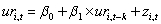 where ur is the state unemployment rate,i is the index for the i-th state,t indicates a time period,and typically k ≥ 10.
(a)Explain why finding a slope estimate of one and an intercept of zero is typically interpreted as evidence of "persistence."
(b)You collect data on the 48 contiguous U.S.states' unemployment rates and find the following estimates:
where ur is the state unemployment rate,i is the index for the i-th state,t indicates a time period,and typically k ≥ 10.
(a)Explain why finding a slope estimate of one and an intercept of zero is typically interpreted as evidence of "persistence."
(b)You collect data on the 48 contiguous U.S.states' unemployment rates and find the following estimates:  = 2.25 + 0.60 ×
  ;R2 = 0.40,SER = 0.90
(0.61)(0.13)
Interpret the regression results.
(c)Analyzing the accompanying figure,and interpret the observation for Maryland and for Washington.Do you find evidence of persistence? How would you test for it?
;R2 = 0.40,SER = 0.90
(0.61)(0.13)
Interpret the regression results.
(c)Analyzing the accompanying figure,and interpret the observation for Maryland and for Washington.Do you find evidence of persistence? How would you test for it? 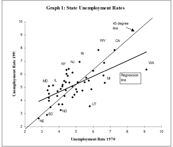 (d)One of your peers points out that this result makes little sense,since it implies that eventually all states would have identical unemployment rates.Explain the argument.
(e)Imagine that state unemployment rates were determined by their natural rates and some transitory shock.The natural rates themselves may be functions of the unemployment insurance benefits of the state,unionization rates of its labor force,demographics,sectoral composition,etc.The transitory components may include state-specific shocks to its terms of trade such as raw material movements and demand shocks from the other states.You specify the i-th state unemployment rate accordingly as follows for the two periods when you observe it,
(d)One of your peers points out that this result makes little sense,since it implies that eventually all states would have identical unemployment rates.Explain the argument.
(e)Imagine that state unemployment rates were determined by their natural rates and some transitory shock.The natural rates themselves may be functions of the unemployment insurance benefits of the state,unionization rates of its labor force,demographics,sectoral composition,etc.The transitory components may include state-specific shocks to its terms of trade such as raw material movements and demand shocks from the other states.You specify the i-th state unemployment rate accordingly as follows for the two periods when you observe it,  so that actual unemployment rates are measured with error.You have also assumed that the natural rate is the same for both periods.Subtracting the second period from the first then results in the following population regression function:
  It is not too hard to show that estimation of the observed unemployment rate in period t on the unemployment rate in period (t-k)by OLS results in an estimator for the slope coefficient that is biased towards zero.The formula is
  .
Using this insight,explain over which periods you would expect the slope to be closer to one,and over which period it should be closer to zero.
(f)Estimating the same regression for a different time period results in
.
Using this insight,explain over which periods you would expect the slope to be closer to one,and over which period it should be closer to zero.
(f)Estimating the same regression for a different time period results in  = 3.19 + 0.27 ×
  ;R2 = 0.21,SER = 1.03
(0.56)(0.07)
If your above analysis is correct,what are the implications for this time period?
;R2 = 0.21,SER = 1.03
(0.56)(0.07)
If your above analysis is correct,what are the implications for this time period?
(Essay)
4.8/5 (37)
Until about 10 years ago,most studies in labor economics found a small but significant negative relationship between minimum wages and employment for teenagers.Two labor economists challenged this perceived wisdom with a publication in 1992 by comparing employment changes of fast-food restaurants in Texas,before and after a federal minimum wage increase.
(a)Explain how you would obtain external validity in this field of study.
(b)List the various threats to external validity and suggest how to address them in this case.
(Essay)
4.9/5 (39)
Consider a situation where Y is related to X in the following manner: Yi = β0 ×  × eui.Draw the deterministic part of the above function.Next add,in the same graph,a hypothetical Y,X scatterplot of the actual observations.Assume that you have misspecified the functional form of the regression function and estimated the relationship between Y and X using a linear regression function.Add this linear regression function to your graph.Separately,show what the plot of the residuals against the X variable in your regression would look like.
(Essay)
5.0/5 (33)
To compare the slope coefficient from the California School data set with that of the Massachusetts School data set,you run the following two regressions:  CA = 2.35 - 0.123×STRCA
(0.54)(0.027)
n = 420,R2 = 0.051,SER = 0.98
CA = 2.35 - 0.123×STRCA
(0.54)(0.027)
n = 420,R2 = 0.051,SER = 0.98  MA = 1.97 - 0.114×STRMA
(0.57)(0.033)
n = 220,R2 = 0.067,SER = 0.97
Numbers in parenthesis are heteroskedasticity-robust standard errors,and the LHS variable has been standardized.
Calculate a t-statistic to test whether or not the two coefficients are the same.State the alternative hypothesis.Which level of significance did you choose?
MA = 1.97 - 0.114×STRMA
(0.57)(0.033)
n = 220,R2 = 0.067,SER = 0.97
Numbers in parenthesis are heteroskedasticity-robust standard errors,and the LHS variable has been standardized.
Calculate a t-statistic to test whether or not the two coefficients are the same.State the alternative hypothesis.Which level of significance did you choose?
(Essay)
4.8/5 (27)
One of the most frequently used summary statistics for the performance of a baseball hitter is the so-called batting average.In essence,it calculates the percentage of hits in the number of opportunities to hit (appearances "at the plate").The management of a professional team has hired you to predict next season's performance of a certain hitter who is up for a contract renegotiation after a particularly great year.To analyze the situation,you search the literature and find a study which analyzed players who had at least 50 at bats in 1998 and 1997.There were 379 such players.
(a)The reported regression line in the study is  = 0.138 + 0.467 ×
  ;R2= 0.17
and the intercept and slope are both statistically significant.What does the regression imply about the relationship between past performance and present performance? What values would the slope and intercept have to take on for the future performance to be as good as the past performance,on average?
(b)Being somewhat puzzled about the results,you call your econometrics professor and describe the results to her.She says that she is not surprised at all,since this is an example of "Galton's Fallacy." She explains that Sir Francis Galton regressed the height of offspring on the mid-height of their parents and found a positive intercept and a slope between zero and one.He referred to this result as "regression towards mediocrity." Why do you think econometricians refer to this result as a fallacy?
(c)Your professor continues by mentioning that this is an example of errors-in-variables bias.What does she mean by that in general? In this case,why would batting averages be measured with error? Are baseball statisticians sloppy?
(d)The top three performers in terms of highest batting averages in 1997 were Tony Gwynn (.372),Larry Walker (.366),and Mike Piazza (.362).Given your answers for the previous questions,what would be your predictions for the 1998 season?
;R2= 0.17
and the intercept and slope are both statistically significant.What does the regression imply about the relationship between past performance and present performance? What values would the slope and intercept have to take on for the future performance to be as good as the past performance,on average?
(b)Being somewhat puzzled about the results,you call your econometrics professor and describe the results to her.She says that she is not surprised at all,since this is an example of "Galton's Fallacy." She explains that Sir Francis Galton regressed the height of offspring on the mid-height of their parents and found a positive intercept and a slope between zero and one.He referred to this result as "regression towards mediocrity." Why do you think econometricians refer to this result as a fallacy?
(c)Your professor continues by mentioning that this is an example of errors-in-variables bias.What does she mean by that in general? In this case,why would batting averages be measured with error? Are baseball statisticians sloppy?
(d)The top three performers in terms of highest batting averages in 1997 were Tony Gwynn (.372),Larry Walker (.366),and Mike Piazza (.362).Given your answers for the previous questions,what would be your predictions for the 1998 season?
(Essay)
4.7/5 (49)
Your textbook gives the following example of simultaneous causality bias of a two equation system:
Yi = β0 + β1Xi + ui
Xi =  +
+  Yi + vi
In microeconomics,you studied the demand and supply of goods in a single market.Let the demand (
Yi + vi
In microeconomics,you studied the demand and supply of goods in a single market.Let the demand (  )and supply (
  )for the i-th good be determined as follows,
  = β0 - β1Pi + ui,
  =
=  -
-  Pi + vi,
where P is the price of the good.In addition,you typically assume that the market clears.
Explain how the simultaneous causality bias applies in this situation.The textbook explained a positive correlation between Xi and ui for
Pi + vi,
where P is the price of the good.In addition,you typically assume that the market clears.
Explain how the simultaneous causality bias applies in this situation.The textbook explained a positive correlation between Xi and ui for  > 0 through an argument that started from "imagine that ui is negative." Repeat this exercise here.
(Essay)
4.9/5 (35)
Give at least three examples where you could envision errors-in-variables problems.For the case where the measurement error occurs only for the explanatory variable in the simple regression case,derive 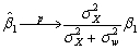 .
.
(Essay)
4.9/5 (28)
Sir Francis Galton (1822-1911),an anthropologist and cousin of Charles Darwin,created the term regression.In his article "Regression towards Mediocrity in Hereditary Stature," Galton compared the height of children to that of their parents,using a sample of 930 adult children and 205 couples.In essence he found that tall (short)parents will have tall (short)offspring,but that the children will not be quite as tall (short)as their parents,on average.Hence there is regression towards the mean,or as Galton referred to it,mediocrity.This result is obviously a fallacy if you attempted to infer behavior over time since,if true,the variance of height in humans would shrink over generations.This is not the case.
(a)To research this result,you collect data from 110 college students and estimate the following relationship:  = 19.6 + 0.73 × Midparh,R2 = 0.45,SER = 2.0
(7.2)(0.10)
where Studenth is the height of students in inches and Midparh is the average of the parental heights.Values in parentheses are heteroskedasticity-robust standard errors.Sketching this regression line together with the 45 degree line,explain why the above results suggest "regression to the mean" or "mean reversion."
(b)Researching the medical literature,you find that height depends,to a large extent,on one gene ("phog")and on environmental influences.Let us assume that parents and offspring have the same invariant (over time)gene and that actual height is therefore measured with error in the following sense,
= 19.6 + 0.73 × Midparh,R2 = 0.45,SER = 2.0
(7.2)(0.10)
where Studenth is the height of students in inches and Midparh is the average of the parental heights.Values in parentheses are heteroskedasticity-robust standard errors.Sketching this regression line together with the 45 degree line,explain why the above results suggest "regression to the mean" or "mean reversion."
(b)Researching the medical literature,you find that height depends,to a large extent,on one gene ("phog")and on environmental influences.Let us assume that parents and offspring have the same invariant (over time)gene and that actual height is therefore measured with error in the following sense,  where
where  is measured height,X is the height given through the gene,v and w are environmental influences,and the subscripts o and p stand for offspring and parents,respectively.Let the environmental influences be independent from each other and from the gene.
Subtracting the measured height of offspring from the height of parents,what sort of population regression function do you expect?
(c)How would you test for the two restrictions implicit in the population regression function in (b)? Can you tell from the results in (a)whether or not the restrictions hold?
(d)Proceeding in a similar way to the proof in your textbook,you can show that
is measured height,X is the height given through the gene,v and w are environmental influences,and the subscripts o and p stand for offspring and parents,respectively.Let the environmental influences be independent from each other and from the gene.
Subtracting the measured height of offspring from the height of parents,what sort of population regression function do you expect?
(c)How would you test for the two restrictions implicit in the population regression function in (b)? Can you tell from the results in (a)whether or not the restrictions hold?
(d)Proceeding in a similar way to the proof in your textbook,you can show that  for the situation in (b).Discuss under what conditions you will find a slope closer to one for the height comparison.Under what conditions will you find a slope closer to zero?
(e)Can you think of other examples where Galton's Fallacy might apply?
for the situation in (b).Discuss under what conditions you will find a slope closer to one for the height comparison.Under what conditions will you find a slope closer to zero?
(e)Can you think of other examples where Galton's Fallacy might apply?
(Essay)
4.9/5 (35)
Filters
- Essay(0)
- Multiple Choice(0)
- Short Answer(0)
- True False(0)
- Matching(0)