Exam 5: Regression With a Single Regressor: Hypothesis Tests and Confidence Intervals

(Continuation from Chapter 4,number 5)You have learned in one of your economics courses that one of the determinants of per capita income (the "Wealth of Nations")is the population growth rate.Furthermore you also found out that the Penn World Tables contain income and population data for 104 countries of the world.To test this theory,you regress the GDP per worker (relative to the United States)in 1990 (RelPersInc)on the difference between the average population growth rate of that country (n)to the U.S.average population growth rate (nus )for the years 1980 to 1990.This results in the following regression output: = 0.518 - 18.831×(n - nus),R2=0.522,SER = 0.197 (0.056)(3.177) (a)Is there any reason to believe that the variance of the error terms is homoskedastic? (b)Is the relationship statistically significant?

(Requires Appendix material)Your textbook shows that OLS is a linear estimator 1 = ,where .For OLS to be conditionally unbiased,the following two conditions must hold: and = 1.Show that this is the case.

The homoskedasticity-only estimator of the variance of 1 is

You have collected data for the 50 U.S.states and estimated the following relationship between the change in the unemployment rate from the previous year ( )and the growth rate of the respective state real GDP (gy).The results are as follows = 2.81 - 0.23 gy,R2= 0.36,SER = 0.78 (0.12)(0.04) Assuming that the estimator has a normal distribution,the 95% confidence interval for the slope is approximately the interval

The p-value for a one-sided left-tail test is given by

Your textbook discussed the regression model when X is a binary variable Yi = β0 + β1Di + ui,i = 1... ,n Let Y represent wages,and let D be one for females,and 0 for males.Using the OLS formula for the slope coefficient,prove that is the difference between the average wage for males and the average wage for females.

The t-statistic is calculated by dividing

(Continuation of the Purchasing Power Parity question from Chapter 4)The news-magazine The Economist regularly publishes data on the so called Big Mac index and exchange rates between countries.The data for 30 countries from the April 29,2000 issue is listed below: Price of Actual Exchange Rate Country Currency Big Mac per U.S.dollar Indonesia Rupiah 14,500 7,945 Italy Lira 4,500 2,088 South Korea Won 3,000 1,108 Chile Peso 1,260 514 Spain Peseta 375 179 Hungary Forint 339 279 Japan Yen 294 106 Taiwan Dollar 70 30.6 Thailand Baht 55 38.0 Czech Rep.Crown 54.37 39.1 Russia Ruble 39.50 28.5 Denmark Crown 24.75 8.04 Sweden Crown 24.0 8.84 Mexico Peso 20.9 9.41 France Franc 18.5 7.07 Israel Shekel 14.5 4.05 China Yuan 9.90 8.28 South Africa Rand 9.0 6.72 Switzerland Franc 5.90 1.70 Poland Zloty 5.50 4.30 Germany Mark 4.99 2.11 Malaysia Dollar 4.52 3.80 New Zealand Dollar 3.40 2.01 Singapore Dollar 3.20 1.70 Brazil Real 2.95 1.79 Canada Dollar 2.85 1.47 Australia Dollar 2.59 1.68 Argentina Peso 2.50 1.00 Britain Pound 1.90 0.63 United States Dollar 2.51 The concept of purchasing power parity or PPP ("the idea that similar foreign and domestic goods … should have the same price in terms of the same currency," Abel,A.and B.Bernanke,Macroeconomics,4th edition,Boston: Addison Wesley,476)suggests that the ratio of the Big Mac priced in the local currency to the U.S.dollar price should equal the exchange rate between the two countries. After entering the data into your spread sheet program,you calculate the predicted exchange rate per U.S.dollar by dividing the price of a Big Mac in local currency by the U.S.price of a Big Mac ($2.51).To test for PPP,you regress the actual exchange rate on the predicted exchange rate. The estimated regression is as follows: = -27.05 + 1.35 × 1.35×Pr edExRate R2 = 0.994,n = 29,SER = 122.15 (23.74)(0.02) (a)Your spreadsheet program does not allow you to calculate heteroskedasticity robust standard errors.Instead,the numbers in parenthesis are homoskedasticity only standard errors.State the two null hypothesis under which PPP holds.Should you use a one-tailed or two-tailed alternative hypothesis? (b)Calculate the two t-statistics. (c)Using a 5% significance level,what is your decision regarding the null hypothesis given the two t-statistics? What critical values did you use? Are you concerned with the fact that you are testing the two hypothesis sequentially when they are supposed to hold simultaneously? (d)What assumptions had to be made for you to use Student's t-distribution?

The neoclassical growth model predicts that for identical savings rates and population growth rates,countries should converge to the per capita income level.This is referred to as the convergence hypothesis.One way to test for the presence of convergence is to compare the growth rates over time to the initial starting level,i.e. ,to run the regression = + × RelProd60 ,where g6090 is the average annual growth rate of GDP per worker for the 1960-1990 sample period,and RelProd60 is GDP per worker relative to the United States in 1960.Under the null hypothesis of no convergence,β1 = 0;H1 : β1 < 0,implying ("beta")convergence.Using a standard regression package,you get the following output: Dependent Variable: G6090 Method: Least Squares Date: 07/11/06 Time: 05:46 Sample: 1 104 Included observations: 104 White Heteroskedasticity-Consistent Standard Errors & Covariance 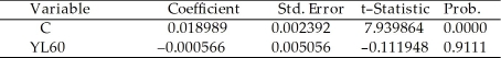You are delighted to see that this program has already calculated p-values for you.However,a peer of yours points out that the correct p-value should be 0.4562.Who is right?

The effect of decreasing the student-teacher ratio by one is estimated to result in an improvement of the districtwide score by 2.28 with a standard error of 0.52.Construct a 90% and 99% confidence interval for the size of the slope coefficient and the corresponding predicted effect of changing the student-teacher ratio by one.What is the intuition on why the 99% confidence interval is wider than the 90% confidence interval?

(continuation from Chapter 4,number 3)You have obtained a sub-sample of 1744 individuals from the Current Population Survey (CPS)and are interested in the relationship between weekly earnings and age.The regression,using heteroskedasticity-robust standard errors,yielded the following result: = 239.16 + 5.20×Age ,R2 = 0.05,SER = 287.21. , (20.24)(0.57) where Earn and Age are measured in dollars and years respectively. (a)Is the relationship between Age and Earn statistically significant? (b)The variance of the error term and the variance of the dependent variable are related.Given the distribution of earnings,do you think it is plausible that the distribution of errors is normal? (c)Construct a 95% confidence interval for both the slope and the intercept.

Using the textbook example of 420 California school districts and the regression of testscores on the student-teacher ratio,you find that the standard error on the slope coefficient is 0.51 when using the heteroskedasticity robust formula,while it is 0.48 when employing the homoskedasticity only formula.When calculating the t-statistic,the recommended procedure is to

The error term is homoskedastic if

(Continuation from Chapter 4)Sir Francis Galton,a cousin of James Darwin,examined the relationship between the height of children and their parents towards the end of the 19th century.It is from this study that the name "regression" originated.You decide to update his findings by collecting data from 110 college students,and estimate the following relationship: = 19.6 + 0.73 × Midparh,R2 = 0.45,SER = 2.0 (7.2)(0.10) where Studenth is the height of students in inches,and Midparh is the average of the parental heights.Values in parentheses are heteroskedasticity robust standard errors.(Following Galton's methodology,both variables were adjusted so that the average female height was equal to the average male height. ) (a)Test for the statistical significance of the slope coefficient. (b)If children,on average,were expected to be of the same height as their parents,then this would imply two hypotheses,one for the slope and one for the intercept. (i)What should the null hypothesis be for the intercept? Calculate the relevant t-statistic and carry out the hypothesis test at the 1% level. (ii)What should the null hypothesis be for the slope? Calculate the relevant t-statistic and carry out the hypothesis test at the 5% level. (c)Can you reject the null hypothesis that the regression R2 is zero? (d)Construct a 95% confidence interval for a one inch increase in the average of parental height.

In order to formulate whether or not the alternative hypothesis is one-sided or two-sided,you need some guidance from economic theory.Choose at least three examples from economics or other fields where you have a clear idea what the null hypothesis and the alternative hypothesis for the slope coefficient should be.Write a brief justification for your answer.

Consider the estimated equation from your textbook =698.9 - 2.28 STR,R2 = 0.051,SER = 18.6 (10.4)(0.52) The t-statistic for the slope is approximately

Consider the sample regression function i = + Xi.The table below lists estimates for the slope ( )and the variance of the slope estimator ( ).In each case calculate the p-value for the null hypothesis of β1 = 0 and a two-tailed alternative hypothesis.Indicate in which case you would reject the null hypothesis at the 5% significance level.

(Continuation from Chapter 4,number 6)The neoclassical growth model predicts that for identical savings rates and population growth rates,countries should converge to the per capita income level.This is referred to as the convergence hypothesis.One way to test for the presence of convergence is to compare the growth rates over time to the initial starting level. (a)The results of the regression for 104 countries were as follows: = 0.019 - 0.0006 × RelProd60,R2= 0.00007,SER = 0.016 (0.004)(0.0073) where g6090 is the average annual growth rate of GDP per worker for the 1960-1990 sample period,and RelProd60 is GDP per worker relative to the United States in 1960.Numbers in parenthesis are heteroskedasticity robust standard errors. Using the OLS estimator with homoskedasticity-only standard errors,the results changed as follows: = 0.019 - 0.0006×RelProd60,R2= 0.00007,SER = 0.016 (0.002)(0.0068) Why didn't the estimated coefficients change? Given that the standard error of the slope is now smaller,can you reject the null hypothesis of no beta convergence? Are the results in the second equation more reliable than the results in the first equation? Explain. (b)You decide to restrict yourself to the 24 OECD countries in the sample.This changes your regression output as follows (numbers in parenthesis are heteroskedasticity robust standard errors): = 0.048 - 0.0404 RelProd60,R2 = 0.82,SER = 0.0046 (0.004)(0.0063) Test for evidence of convergence now.If your conclusion is different than in (a),speculate why this is the case. (c)The authors of your textbook have informed you that unless you have more than 100 observations,it may not be plausible to assume that the distribution of your OLS estimators is normal.What are the implications here for testing the significance of your theory?

Using the California School data set from your textbook,you run the following regression: = 698.9 - 2.28 STR n = 420,R2 = 0.051,SER = 18.6 where TestScore is the average test score in the district and STR is the student-teacher ratio.Using heteroskedasticity robust standard errors,you find while choosing the homoskedasticity-only option,the standard error is 0.48. a.Calculate the t-statistic for both standard errors. b.Which of the two t-statistics should you base your inference on?

Your textbook states that under certain restrictive conditions,the t- statistic has a Student t-distribution with n-2 degrees of freedom.The loss of two degrees of freedom is the result of OLS forcing two restrictions onto the data.What are these two conditions,and when did you impose them onto the data set in your derivation of the OLS estimator?