Exam 15: Estimation of Dynamic Causal Effects

Money supply is linked to the monetary base by the money multiplier.Macroeconomic textbooks tell you that the central bank cannot control the money supply,but it can control the monetary base.As a result,you decide to specify a distributed lag equation of the growth in the money supply on the growth in the monetary base.One of your peers tells you that this is not a good idea for modeling the relationship between the two variables.What does she mean?

Estimation of dynamic multipliers under strict exogeneity should be done by

Sensitivity analysis of the results may include the following with the exception of

The distributed lag model relating orange juice prices to the Orlando weather reported in the text was of the form %ChgPt = β0 + β1FDDt + β2FDDt-1 + β3FDDt-2 + ...+ β19FDDt-18 + ut (a)Suppose that an agricultural economist tells you that a freeze in December is more harmful than a freeze in the other months.How would you modify the regression to incorporate this effect? How would you test for this December effect? (b)The same economist tells you that the damage caused by freezes is not well captured by the FDD variable.She says that a single day temperature with a temperature of 24° is more damaging than 8 days with a temperature of 31°.How would you modify the regression to incorporate this effect?

Consider the following distributed lag model is serially uncorrelated,and X is strictly exogenous. (a)How many parameters are there to be estimated between the two equations? (b)Using the two equations of the model above,derive the ADL form of the model. (c)There are five regressors in the ADL model,namely Yt-1,Xt,Xt-1,Xt-2 and the constant.Estimating the ADL model linearly will give you five coefficients.Can you derive the parameters of the original two equation model from these five estimates? Why or why not? (d)What alternative method do you have to retrieve the parameters of the two equation model?

The long-run cumulative dynamic multiplier

To convey information about the dynamic multipliers more effectively,you should

There is some economic research which suggests that oil prices play a central role in causing recessions in developed countries.Some of this work suggests that it is only oil price increases that matter and even more specifically,that it is the percentage point difference between oil prices at date t and the maximum value over the previous year.Realizing that energy prices in general can fluctuate quite dramatically in both directions and that geographic areas also benefit substantially from oil price decreases,you decide to estimate the following distributed lag model using annual data (numbers in parenthesis are HAC standard errors): t = 3.39 - 0.009 (Poil/CPI)t - 0.028 (Poil/CPI)t-1 (0.27)(0.010)(0.011) t = 1960-2008,R2 = 0.15,SER = 1.88 a.What is the impact effect of a 25 percent increase in real oil prices? b.What is the predicted cumulative change in GDP Growth over two years of this effect? c.The HAC F-statistic is 4.07.Can you reject the null hypothesis that oil price changes have no effect on real GDP growth? What is the critical value you considered? Is there any reason why you should be cautious using an F-test in this case,given the sample period?

The distributed lag regression model requires estimation of (r+1)coefficients in the case of a single explanatory variable.In your textbook example of orange juice prices and cold weather,r = 18.With additional explanatory variables,this number becomes even larger. Consider the distributed lag regression model with a single regressor Yt = β0 + β1Xt + β2Xt-1 + β3Xt-2 + ...+ βr+1Xt-r + ut (a)Early econometric analysis of distributed lag regression models was interested in reducing the number of parameters by approximating the coefficients by a polynomial of a suitable degree,i.e. ,βi+1 ≈ f(i)for i = 0,1,…,r.Let f(i)be a third degree polynomial,with coefficients α0,.... ,α3.Specify the equations for β1,β2,β3,β4,and βr+1. (b)Substitute these equations into the original distributed lag regression,and rearrange terms so that Y appears as a linear function of β0,α0,α1,α2,α3 and a transformation of the Xt,Xt-1,Xt-2,... ,Xt-r (c)Assume that the third-degree polynomial approximation is quite accurate.Then what is the advantage of this polynomial lag technique?

Quasi differences in Yt are defined as

The distributed lag model is given by

Ascertaining whether or not a regressor is strictly exogenous or exogenous ultimately requires all of the following with the exception of

Your textbook presents as an example of a distributed lag regression the effect of the weather on the price of orange juice.The authors mention U.S.income and Australian exports,oil prices and inflation,monetary policy and inflation,and the Phillips curve as other candidates for distributed lag regression.Briefly discuss whether or not the exogeneity assumption is likely to hold in each of these cases.Explain why it is so hard to come up with good examples of distributed lag regressions in economics.

A distributed lag regression

Your textbook estimates the initial relationship between the percentage change of real frozen OJ and the freezing degree days as follows: t = -0.40 + 0.47 FDDt (0.22)(0.13) t = 1950:1 - 2000:12,R2 = 0.09,SER = 4.8 a.Calculate the t-statistic for the slope coefficient.Can you reject the null hypothesis that the coefficient is zero in the population? b.The above regression was estimated using HAC standard errors.When you re-estimate the regression using homoskedasticity-only standard errors,the standard error of the slope coefficient drops to 0.06.Calculate the t-statistic for the slope coefficient again.Which of the two standard errors should you use for statistical inference?

One of the central predictions of neo-classical macroeconomic growth theory is that an increase in the growth rate of the population causes at first a decline the growth rate of real output per capita,but that subsequently the growth rate returns to its natural level,itself determined by the rate of technological innovation.The intuition is that,if the growth rate of the workforce increases,then more has to be saved to provide the new workers with physical capital.However,accumulating capital takes time,so that output per capita falls in the short run. Under the assumption that population growth is exogenous,a number of regressions of the growth rate of output per capita on current and lagged population growth were performed,as reported below.(A constant was included in the regressions but is not reported.HAC standard errors are in brackets.BIC is listed at the bottom of the table). Regression of Growth Rate of Real Per-Capita GDP on Lags of Population Growth, United States,1825-2000 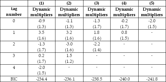(a)Which of these models is favored by the information criterion? (b)How consistent are these estimates with the theory? Is this a fair test of the theory? Why or why not? (c)Can you think of any improved data to test the theory?

A model that attracted quite a bit of interest in macroeconomics in the 1970s was the St.Louis model.The underlying idea was to calculate fiscal and monetary impact and long run cumulative dynamic multipliers,by relating output (growth)to government expenditure (growth)and money supply (growth).The assumption was that both government expenditures and the money supply were exogenous.Estimation of a St.Louis type model using quarterly data from 1960:I-1995:IV results in the following output (HAC standard errors in parenthesis): t = 0.018 + 0.006 × dmgrowtht + 0.235 × dmgrowtht-1 + 0.344 × dmgrowtht-2 (0.004)(0.079)(0.091)(0.087) + 0.385 × dmgrotht-3 + 0.425 × mgrowtht-4 + 0.170 × dggrowtht - 0.044dggrowtht-1 (0.097)(0.069)(0.049)(0.068) - 0.003 × dggrowtht-2 - 0.079 × dggrowtht-3 + 0.018 × ggrowtht-4; (0.040)(0.051)(0.027) R2 = 0.346,SER=0.03 where ygrowth is quarterly growth of real GDP,mgrowth is quarterly growth of real money supply (M2),and ggrowth is quarterly growth of real government expenditures."d" in front of ggrowth and mgrowth indicates a change in the variable. (a)Assuming that money and government expenditures are exogenous,what do the coefficients represent? Calculate the h-period cumulative dynamic multipliers from these.How can you test for the statistical significance of the cumulative dynamic multipliers and the long-run cumulative dynamic multiplier? (b)Sketch the estimated dynamic and cumulative dynamic fiscal and monetary multipliers. (c)For these coefficients to represent dynamic multipliers,the money supply and government expenditures must be exogenous variables.Explain why this is unlikely to be the case.As a result,what importance should you attach to the above results?

Given the relationship between the two variables,the following is most likely to be exogenous:

In time series data,it is useful to think of a randomized controlled experiment

To estimate dynamic causal effects,your textbook presents the distributed lag regression model,the autoregressive distributed lag model,and a quasi-difference representation of the distributed lag model with autoregressive errors.Using a simple example,such as a distributed lag model with only the current and past value of X and an AR(1)model for the error term,discuss how these models are related.In each case suggest estimation methods and evaluate the relative merit in using one rather than the other.