Exam 8: Nonlinear Regression Functions
Pages 283-284 in your textbook contain an analysis of the "Return to Education and the Gender Gap." Column (4)in Table 8.1 displays regression results using the 2009 Current Population Survey.The equation below shows the regression result for the same specification,but using the 2005 Current Population Survey.Interpret the major results.  = 1.215 + 0.0899 × educ - 0.521 × DFemme+ 0.0180 × (DFemme×educ)
(0.018)(0.0011)(0.022)(0.0016)
+ 0.0232 × exper - 0.000368 × exper2 - 0.058 × Midwest - 0.0098 × South - 0.030 × West
(0.0008)(0.000018)(0.006)(0.0078)(0.0030)
= 1.215 + 0.0899 × educ - 0.521 × DFemme+ 0.0180 × (DFemme×educ)
(0.018)(0.0011)(0.022)(0.0016)
+ 0.0232 × exper - 0.000368 × exper2 - 0.058 × Midwest - 0.0098 × South - 0.030 × West
(0.0008)(0.000018)(0.006)(0.0078)(0.0030)
The return to education for males is approximately 9% and its coefficient has a t-statistic of 11.25.For females,the return is slightly higher,approximately 11%.Since the binary variable for females is interacted with the number of years of education,the gender gap depends on the number of years of education.For the typical high school graduate (12 years of education),the gender gap is approximately 27%,while for the typical college graduate (16 years of education)the gender gap narrows to 19%.The potential experience variable enters in an inverted U-shape,which is to be expected given the shape of age-earnings profiles and the fact that potential experience depends on the age of the individual.There is a declining marginal value for each year of potential experience until it eventually becomes negative.Northeast is the omitted region,and all other regions have lower (log)earnings,ranging from 0.8% in the South to 5.8% in the Midwest.All coefficients are statistically significant.
8.3 Mathematical and Graphical Problems
Consider the following least squares specification between testscores and the student-teacher ratio:  = 557.8 + 36.42 ln (Income).According to this equation,a 1% increase income is associated with an increase in test scores of
A
In the case of perfect multicollinearity,OLS is unable to estimate the slope coefficients of the variables involved.Assume that you have included both X1 and X2 as explanatory variables,and that X2 = X  ,so that there is an exact relationship between two explanatory variables.Does this pose a problem for estimation?
There is no problem for estimation,since the second explanatory variable is not linearly related to the first.This is an example of a polynomial regression model of degree 2,which is frequently estimated in econometrics
Consider a typical beta convergence regression function from macroeconomics,where the growth of a country's per capita income is regressed on the initial level of per capita income and various other economic and socio-economic variables.Assume that two of these variables are the average number of years of education in the specific country and a binary variable which indicates whether or not the country experienced a significant number of years of civil war/unrest.Explain why it would make sense to have these two variables enter separately and also why you should use an interaction term.What signs would you expect on the three coefficients?
You have learned that earnings functions are one of the most investigated relationships in economics.These typically relate the logarithm of earnings to a series of explanatory variables such as education,work experience,gender,race,etc.
(a)Why do you think that researchers have preferred a log-linear specification over a linear specification? In addition to the interpretation of the slope coefficients,also think about the distribution of the error term.
(b)To establish age-earnings profiles,you regress ln(Earn)on Age,where Earn is weekly earnings in dollars,and Age is in years.Plotting the residuals of the regression against age for 1,744 individuals looks as shown in the figure:  Do you sense a problem?
(c)You decide,given your knowledge of age-earning profiles,to allow the regression line to differ for the below and above 40 years age category.Accordingly you create a binary variable,Dage,that takes the value one for age 39 and below,and is zero otherwise.Estimating the earnings equation results in the following output (using heteroskedasticity-robust standard errors):
Do you sense a problem?
(c)You decide,given your knowledge of age-earning profiles,to allow the regression line to differ for the below and above 40 years age category.Accordingly you create a binary variable,Dage,that takes the value one for age 39 and below,and is zero otherwise.Estimating the earnings equation results in the following output (using heteroskedasticity-robust standard errors):  = 6.92 - 3.13 × Dage - 0.019 × Age + 0.085 × (Dage × Age),R2=0.20,SER =0.721.
(38.33)(0.22)(0.004)(0.005)
Sketch both regression lines: one for the age category 39 years and under,and one for 40 and above.Does it make sense to have a negative sign on the Age coefficient? Predict the ln(earnings)for a 30 year old and a 50 year old.What is the percentage difference between these two?
(d)The F-statistic for the hypothesis that both slopes and intercepts are the same is 124.43.Can you reject the null hypothesis?
(e)What other functional forms should you consider?
= 6.92 - 3.13 × Dage - 0.019 × Age + 0.085 × (Dage × Age),R2=0.20,SER =0.721.
(38.33)(0.22)(0.004)(0.005)
Sketch both regression lines: one for the age category 39 years and under,and one for 40 and above.Does it make sense to have a negative sign on the Age coefficient? Predict the ln(earnings)for a 30 year old and a 50 year old.What is the percentage difference between these two?
(d)The F-statistic for the hypothesis that both slopes and intercepts are the same is 124.43.Can you reject the null hypothesis?
(e)What other functional forms should you consider?
Many countries that experience hyperinflation do not have market-determined interest rates.As a result,some authors have substituted future inflation rates into money demand equations of the following type as a proxy:  (m is real money,and P is the consumer price index).
Income is typically omitted since movements in it are dwarfed by money growth and the inflation rate.Authors have then interpreted β1 as the "semi-elasticity" of the inflation rate.Do you see any problems with this interpretation?
(m is real money,and P is the consumer price index).
Income is typically omitted since movements in it are dwarfed by money growth and the inflation rate.Authors have then interpreted β1 as the "semi-elasticity" of the inflation rate.Do you see any problems with this interpretation?
Assume that you had data for a cross-section of 100 households with data on consumption and personal disposable income.If you fit a linear regression function regressing consumption on disposable income,what prior expectations do you have about the slope and the intercept? The slope of this regression function is called the "marginal propensity to consume." If,instead,you fit a log-log model,then what is the interpretation of the slope? Do you have any prior expectation about its size?
An extension of the Solow growth model that includes human capital in addition to physical capital, suggests that investment in human capital (education) will increase the wealth of a nation (per capita income). To test this hypothesis, you collect data for 104 countries and perform the following regression:
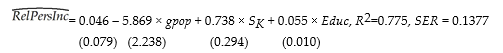 where RelPersInc is GDP per worker relative to the United States, gpop is the average population growth rate, 1980 to 1990, sK is the average investment share of GDP from 1960 to 1990, and Educ is the average educational attainment in years for 1985. Numbers in parentheses are for heteroskedasticity-robust standard errors.
(a) Interpret the results and indicate whether or not the coefficients are significantly different from zero. Do the coefficients have the expected sign?
(b) To test for equality of the coefficients between the OECD and other countries, you introduce a binary variable (DOECD), which takes on the value of one for the OECD countries and is zero otherwise. To conduct the test for equality of the coefficients, you estimate the following regression:
where RelPersInc is GDP per worker relative to the United States, gpop is the average population growth rate, 1980 to 1990, sK is the average investment share of GDP from 1960 to 1990, and Educ is the average educational attainment in years for 1985. Numbers in parentheses are for heteroskedasticity-robust standard errors.
(a) Interpret the results and indicate whether or not the coefficients are significantly different from zero. Do the coefficients have the expected sign?
(b) To test for equality of the coefficients between the OECD and other countries, you introduce a binary variable (DOECD), which takes on the value of one for the OECD countries and is zero otherwise. To conduct the test for equality of the coefficients, you estimate the following regression:
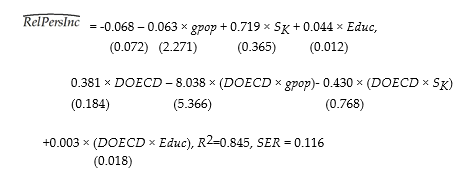 Write down the two regression functions, one for the OECD countries, the other for the non-OECD countries. The F- statistic that all coefficients involving DOECD are zero, is 6.76. Find the corresponding critical value from the F table and decide whether or not the coefficients are equal across the two sets of countries.
(c) Given your answer in the previous question, you want to investigate further. You first force the same slopes across all countries, but allow the intercept to differ. That is, you reestimate the above regression
Write down the two regression functions, one for the OECD countries, the other for the non-OECD countries. The F- statistic that all coefficients involving DOECD are zero, is 6.76. Find the corresponding critical value from the F table and decide whether or not the coefficients are equal across the two sets of countries.
(c) Given your answer in the previous question, you want to investigate further. You first force the same slopes across all countries, but allow the intercept to differ. That is, you reestimate the above regression
 The t-statistic for DOECD is 4.39. Is the coefficient, which was 0.241, statistically significant?
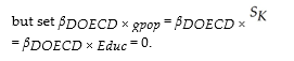
(d) Your final regression allows the slopes to differ in addition to the intercept. The F-statistic for
The t-statistic for DOECD is 4.39. Is the coefficient, which was 0.241, statistically significant?
(d) Your final regression allows the slopes to differ in addition to the intercept. The F-statistic for
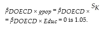 What is your decision? Each one of the t-statistics is also smaller than the critical value from the standard normal table. Which test should you use?
(e) Looking at the tests in the two previous questions, what is your conclusion?
What is your decision? Each one of the t-statistics is also smaller than the critical value from the standard normal table. Which test should you use?
(e) Looking at the tests in the two previous questions, what is your conclusion?
The interpretation of the slope coefficient in the model Yi = β0 + β1 ln(Xi)+ ui is as follows:
One of the most frequently estimated equations in the macroeconomics growth literature are so-called convergence regressions.In essence the average per capita income growth rate is regressed on the beginning-of-period per capita income level to see if countries that were further behind initially,grew faster.Some macroeconomic models make this prediction,once other variables are controlled for.To investigate this matter,you collect data from 104 countries for the sample period 1960-1990 and estimate the following relationship (numbers in parentheses are for heteroskedasticity-robust standard errors):  = 0.020 - 0.360 × gpop + 0.00 4 × Educ - 0.053×RelProd60,R2=0.332,SER = 0.013
(0.009)(0.241)(0.001)(0.009)
where g6090 is the growth rate of GDP per worker for the 1960-1990 sample period,RelProd60 is the initial starting level of GDP per worker relative to the United States in 1960,gpop is the average population growth rate of the country,and Educ is educational attainment in years for 1985.
(a)What is the effect of an increase of 5 years in educational attainment? What would happen if a country could implement policies to cut population growth by one percent? Are all coefficients significant at the 5% level? If one of the coefficients is not significant,should you automatically eliminate its variable from the list of explanatory variables?
(b)The coefficient on the initial condition has to be significantly negative to suggest conditional convergence.Furthermore,the larger this coefficient,in absolute terms,the faster the convergence will take place.It has been suggested to you to interact education with the initial condition to test for additional effects of education on growth.To test for this possibility,you estimate the following regression:
= 0.020 - 0.360 × gpop + 0.00 4 × Educ - 0.053×RelProd60,R2=0.332,SER = 0.013
(0.009)(0.241)(0.001)(0.009)
where g6090 is the growth rate of GDP per worker for the 1960-1990 sample period,RelProd60 is the initial starting level of GDP per worker relative to the United States in 1960,gpop is the average population growth rate of the country,and Educ is educational attainment in years for 1985.
(a)What is the effect of an increase of 5 years in educational attainment? What would happen if a country could implement policies to cut population growth by one percent? Are all coefficients significant at the 5% level? If one of the coefficients is not significant,should you automatically eliminate its variable from the list of explanatory variables?
(b)The coefficient on the initial condition has to be significantly negative to suggest conditional convergence.Furthermore,the larger this coefficient,in absolute terms,the faster the convergence will take place.It has been suggested to you to interact education with the initial condition to test for additional effects of education on growth.To test for this possibility,you estimate the following regression:  = 0.015 - 0.323 × gpop + 0.005 × Educ - 0.051 × RelProd60
(0.009)(0.238)(0.001)(0.013)
-0.0028 × (EducRelProd60),R2=0.346,SER = 0.013
(0.0015)
Write down the effect of an additional year of education on growth.West Germany has a value for RelProd60 of 0.57,while Brazil's value is 0.23.What is the predicted growth rate effect of adding one year of education in both countries? Does this predicted growth rate make sense?
(c)What is the implication for the speed of convergence? Is the interaction effect statistically significant?
(d)Convergence regressions are basically of the type
Δln Yt = β0 - β1 ln Y0
where △ might be the change over a longer time period,30 years,say,and the average growth rate is used on the left-hand side.You note that the equation can be rewritten as
△ln Yt = β0 - (1 - β1)ln Y0
Over a century ago,Sir Francis Galton first coined the term "regression" by analyzing the relationship between the height of children and the height of their parents.Estimating a function of the type above,he found a positive intercept and a slope between zero and one.He therefore concluded that heights would revert to the mean.Since ultimately this would imply the height of the population being the same,his result has become known as "Galton's Fallacy." Your estimate of β1 above is approximately 0.05.Do you see a parallel to Galton's Fallacy?
= 0.015 - 0.323 × gpop + 0.005 × Educ - 0.051 × RelProd60
(0.009)(0.238)(0.001)(0.013)
-0.0028 × (EducRelProd60),R2=0.346,SER = 0.013
(0.0015)
Write down the effect of an additional year of education on growth.West Germany has a value for RelProd60 of 0.57,while Brazil's value is 0.23.What is the predicted growth rate effect of adding one year of education in both countries? Does this predicted growth rate make sense?
(c)What is the implication for the speed of convergence? Is the interaction effect statistically significant?
(d)Convergence regressions are basically of the type
Δln Yt = β0 - β1 ln Y0
where △ might be the change over a longer time period,30 years,say,and the average growth rate is used on the left-hand side.You note that the equation can be rewritten as
△ln Yt = β0 - (1 - β1)ln Y0
Over a century ago,Sir Francis Galton first coined the term "regression" by analyzing the relationship between the height of children and the height of their parents.Estimating a function of the type above,he found a positive intercept and a slope between zero and one.He therefore concluded that heights would revert to the mean.Since ultimately this would imply the height of the population being the same,his result has become known as "Galton's Fallacy." Your estimate of β1 above is approximately 0.05.Do you see a parallel to Galton's Fallacy?
In the model ln(Yi)= β0 + β1Xi + ui,the elasticity of E(Y|X)with respect to X is
You have estimated the following equation:  = 607.3 + 3.85 Income - 0.0423 Income2, where TestScore is the average of the reading and math scores on the Stanford 9 standardized test administered to 5th grade students in 420 California school districts in 1998 and 1999.Income is the average annual per capita income in the school district,measured in thousands of 1998 dollars.The equation
Labor economists have extensively researched the determinants of earnings.Investment in human capital,measured in years of education,and on the job training are some of the most important explanatory variables in this research.You decide to apply earnings functions to the field of sports economics by finding the determinants for baseball pitcher salaries.You collect data on 455 pitchers for the 1998 baseball season and estimate the following equation using OLS and heteroskedasticity-robust standard errors:  = 12.45 + 0.052 × Years + 0.00089 × Innings + 0.0032 × Saves
(0.08)(0.026)(0.00020)(0.0018)
- 0.0085 × ERA,R2 = 0.45,SER = 0.874
(0.0168)
where Earn is annual salary in dollars,Years is number of years in the major leagues,Innings is number of innings pitched during the career before the 1998 season,Saves is number of saves during the career before the 1998 season,and ERA is the earned run average before the 1998 season.
(a)What happens to earnings when the pitcher stays in the league for one additional year? Compare the salaries of two relievers,one with 10 more saves than the other.What effect does pitching 100 more innings have on the salary of the pitcher? What effect does reducing his ERA by 1.5? Do the signs correspond to your expectations? Explain.
(b)Are the individual coefficients statistically significant? Indicate the level of significance you used and the type of alternative hypothesis you considered.
(c)Although you are quite impressed with the fit of the regression,someone suggests that you should include the square of years and innings as additional explanatory variables.Your results change as follows:
= 12.45 + 0.052 × Years + 0.00089 × Innings + 0.0032 × Saves
(0.08)(0.026)(0.00020)(0.0018)
- 0.0085 × ERA,R2 = 0.45,SER = 0.874
(0.0168)
where Earn is annual salary in dollars,Years is number of years in the major leagues,Innings is number of innings pitched during the career before the 1998 season,Saves is number of saves during the career before the 1998 season,and ERA is the earned run average before the 1998 season.
(a)What happens to earnings when the pitcher stays in the league for one additional year? Compare the salaries of two relievers,one with 10 more saves than the other.What effect does pitching 100 more innings have on the salary of the pitcher? What effect does reducing his ERA by 1.5? Do the signs correspond to your expectations? Explain.
(b)Are the individual coefficients statistically significant? Indicate the level of significance you used and the type of alternative hypothesis you considered.
(c)Although you are quite impressed with the fit of the regression,someone suggests that you should include the square of years and innings as additional explanatory variables.Your results change as follows:  = 12.15 + 0.160 × Years + 0.00268 × Innings + 0.0063 × Saves
(0.05)(0.039)(0.00030)(0.0010)
- 0.0584 × ERA - 0.0165 × Years2 - 0.00000045 × Innings2
(0.0165)(0.0026)(0.00000012)
R2 = 0.69,SER = 0.666
What is her reasoning? Are the coefficients of the quadratic terms statistically significant? Are they meaningful?
(d)Calculate the effect of moving from two to three years,as opposed to from 12 to 13 years.
(e)You also decide to test the specification for stability across leagues (National League and American League)by including a dummy variable for the National League and allowing the intercept and all slopes to differ.The resulting F-statistic for restricting all coefficients that involve the National League dummy variable to zero,is 0.40.Compare this to the relevant critical value from the table and decide whether or not these additional variables should be included.
= 12.15 + 0.160 × Years + 0.00268 × Innings + 0.0063 × Saves
(0.05)(0.039)(0.00030)(0.0010)
- 0.0584 × ERA - 0.0165 × Years2 - 0.00000045 × Innings2
(0.0165)(0.0026)(0.00000012)
R2 = 0.69,SER = 0.666
What is her reasoning? Are the coefficients of the quadratic terms statistically significant? Are they meaningful?
(d)Calculate the effect of moving from two to three years,as opposed to from 12 to 13 years.
(e)You also decide to test the specification for stability across leagues (National League and American League)by including a dummy variable for the National League and allowing the intercept and all slopes to differ.The resulting F-statistic for restricting all coefficients that involve the National League dummy variable to zero,is 0.40.Compare this to the relevant critical value from the table and decide whether or not these additional variables should be included.
(Requires Calculus)In the equation  = 607.3 + 3.85 Income - 0.0423Income2,the following income level results in the maximum test score
Suggest a transformation in the variables that will linearize the deterministic part of the population regression functions below.Write the resulting regression function in a form that can be estimated by using OLS.
(a)Yi = β0 
 (b)Yi =
  (c)Yi =
  (d)Yi = β0

To test whether or not the population regression function is linear rather than a polynomial of order r,
You have estimated an earnings function,where you regressed the log of earnings on a set of continuous explanatory variables (in levels)and two binary variables,one for gender and the other for marital status.One of the explanatory variables is education.
(a)Interpret the education coefficient.
(b)Next,specify the binary variables and an equation,where the default is a single male,without allowing for interaction between marital status and gender.Indicate the coefficients that measure the effect of a single male,single female,married male,and married female.
(c)Finally allow for an interaction between the gender and marital status binary variables.Repeat the exercise of writing down the various effects based on the female/male and single/married status.Why is the latter approach more general than the former?
The following interactions between binary and continuous variables are possible,with the exception of
To investigate whether or not there is discrimination against a sub-group of individuals,you regress the log of earnings on determining variables,such as education,work experience,etc. ,and a binary variable which takes on the value of one for individuals in that sub-group and is zero otherwise.You consider two possible specifications.First you run two separate regressions,one for the observations that include the sub-group and one for the others.Second,you run a single regression,but allow for a binary variable to appear in the regression.Your professor suggests that the second equation is better for the task at hand,as long as you allow for a shift in both the intercept and the slopes.Explain her reasoning.
(Requires Calculus)Show that for the log-log model the slope coefficient is the elasticity.
Filters
- Essay(0)
- Multiple Choice(0)
- Short Answer(0)
- True False(0)
- Matching(0)