Exam 4: Linear Regression With One Regressor
Prove that the regression R2 is identical to the square of the correlation coefficient between two variables Y and X.Regression functions are written in a form that suggests causation running from X to Y.Given your proof,does a high regression R2 present supportive evidence of a causal relationship? Can you think of some regression examples where the direction of causality is not clear? Is without a doubt?
The regression R2 =  ,where ESS is given by
  .But
.But  i =
i =  0 +
0 +  1Xi and
  =
=  0 +
0 +  1
1  .Hence (
  i -
i -  )2 =
)2 =  (Xi -
(Xi -  )2 and therefore ESS =
 .Using small letters to indicate deviations from mean,i.e. ,zi = Zi -
  ,we get that the regression R2 =
  .The square of the correlation coefficient is
 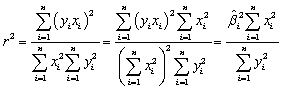 .Hence the two are the same.Correlation does not imply causation.Income is a regressor in the consumption function,yet consumption enters on the right-hand side of the GDP identity.Regressing the weight of individuals on the height is a situation where causality is without doubt,since the author of this test bank should be seven feet tall otherwise.The authors of the textbook use weather data to forecast orange juice prices later in the text.
Assume that there is a change in the units of measurement on X.The new variables X* = bX.Prove that this change in the units of measurement on the explanatory variable has no effect on the intercept in the resulting regression.
Consider the sample regression function  .The formula for the intercept will be
  .But
.But 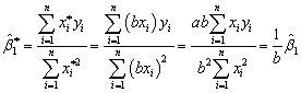 .Hence
  .
.
Your textbook presented you with the following regression output:  = 698.9 - 2.28 × STR
n = 420,R2 = 0.051,SER = 18.6
(a)How would the slope coefficient change,if you decided one day to measure testscores in 100s,i.e. ,a test score of 650 became 6.5? Would this have an effect on your interpretation?
(b)Do you think the regression R2 will change? Why or why not?
(c)Although Chapter 4 in your textbook did not deal with hypothesis testing,it presented you with the large sample distribution for the slope and the intercept estimator.Given the change in the units of measurement in (a),do you think that the variance of the slope estimator will change numerically? Why or why not?
= 698.9 - 2.28 × STR
n = 420,R2 = 0.051,SER = 18.6
(a)How would the slope coefficient change,if you decided one day to measure testscores in 100s,i.e. ,a test score of 650 became 6.5? Would this have an effect on your interpretation?
(b)Do you think the regression R2 will change? Why or why not?
(c)Although Chapter 4 in your textbook did not deal with hypothesis testing,it presented you with the large sample distribution for the slope and the intercept estimator.Given the change in the units of measurement in (a),do you think that the variance of the slope estimator will change numerically? Why or why not?
(a)The new regression line would be  = 6.989 - 0.0228 × STR.Hence the decimal point would simply move two digits to the left.The interpretation remains the same,since an increase in the student-teacher ratio by 2,say,increases the new testscore by 0.0456 points on the new testscore scale,which is 4.56 in the original testscores.
(b)The regression R2 should not change,since,if it did,an objective measure of fit would depend on whim (the units of measurement).The SER will change (from 18.6 to 0.186).This is to be expected,since the TSS obviously changes,and with the regression R2 unchanged,the SSR (and hence SER)have to adjust accordingly.
(c)Since statistical inference will depend on the ratio of the estimator and its standard error,the standard error must change in proportion to the estimator.If this was not true,then statistical inference again would depend on the whim of the investigator.
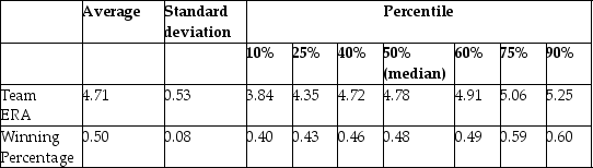
The baseball team nearest to your home town is,once again,not doing well.Given that your knowledge of what it takes to win in baseball is vastly superior to that of management,you want to find out what it takes to win in Major League Baseball (MLB).You therefore collect the winning percentage of all 30 baseball teams in MLB for 1999 and regress the winning percentage on what you consider the primary determinant for wins,which is quality pitching (team earned run average).You find the following information on team performance:
Summary of the Distribution of Winning Percentage and
Team Earned Run Average for MLB in 1999
 (a)What is your expected sign for the regression slope? Will it make sense to interpret the intercept? If not,should you omit it from your regression and force the regression line through the origin?
(b)OLS estimation of the relationship between the winning percentage and the team ERA yield the following:
(a)What is your expected sign for the regression slope? Will it make sense to interpret the intercept? If not,should you omit it from your regression and force the regression line through the origin?
(b)OLS estimation of the relationship between the winning percentage and the team ERA yield the following:  = 0.9 - 0.10 × teamera ,R2=0.49,SER = 0.06,
where winpct is measured as wins divided by games played,so for example a team that won half of its games would have Winpct = 0.50.Interpret your regression results.
(c)It is typically sufficient to win 90 games to be in the playoffs and/or to win a division.Winning over 100 games a season is exceptional: the Atlanta Braves had the most wins in 1999 with 103.Teams play a total of 162 games a year.Given this information,do you consider the slope coefficient to be large or small?
(d)What would be the effect on the slope,the intercept,and the regression R2 if you measured Winpct in percentage points,i.e. ,as (Wins/Games)× 100?
(e)Are you impressed with the size of the regression R2? Given that there is 51% of unexplained variation in the winning percentage,what might some of these factors be?
= 0.9 - 0.10 × teamera ,R2=0.49,SER = 0.06,
where winpct is measured as wins divided by games played,so for example a team that won half of its games would have Winpct = 0.50.Interpret your regression results.
(c)It is typically sufficient to win 90 games to be in the playoffs and/or to win a division.Winning over 100 games a season is exceptional: the Atlanta Braves had the most wins in 1999 with 103.Teams play a total of 162 games a year.Given this information,do you consider the slope coefficient to be large or small?
(d)What would be the effect on the slope,the intercept,and the regression R2 if you measured Winpct in percentage points,i.e. ,as (Wins/Games)× 100?
(e)Are you impressed with the size of the regression R2? Given that there is 51% of unexplained variation in the winning percentage,what might some of these factors be?
Indicate in a scatterplot what the data for your dependent variable and your explanatory variable would look like in a regression with an R2 equal to zero.How would this change if the regression R2 was equal to one?
In order to calculate the slope,the intercept,and the regression R2 for a simple sample regression function,list the five sums of data that you need.
(Requires Calculus)Consider the following model:
Yi = β0 + ui.
Derive the OLS estimator for β0.
Sir Francis Galton,a cousin of James Darwin,examined the relationship between the height of children and their parents towards the end of the 19th century.It is from this study that the name "regression" originated.You decide to update his findings by collecting data from 110 college students,and estimate the following relationship:  = 19.6 + 0.73 × Midparh,R2 = 0.45,SER = 2.0
where Studenth is the height of students in inches,and Midparh is the average of the parental heights.(Following Galton's methodology,both variables were adjusted so that the average female height was equal to the average male height. )
(a)Interpret the estimated coefficients.
(b)What is the meaning of the regression R2?
(c)What is the prediction for the height of a child whose parents have an average height of 70.06 inches?
(d)What is the interpretation of the SER here?
(e)Given the positive intercept and the fact that the slope lies between zero and one,what can you say about the height of students who have quite tall parents? Those who have quite short parents?
(f)Galton was concerned about the height of the English aristocracy and referred to the above result as "regression towards mediocrity." Can you figure out what his concern was? Why do you think that we refer to this result today as "Galton's Fallacy"?
= 19.6 + 0.73 × Midparh,R2 = 0.45,SER = 2.0
where Studenth is the height of students in inches,and Midparh is the average of the parental heights.(Following Galton's methodology,both variables were adjusted so that the average female height was equal to the average male height. )
(a)Interpret the estimated coefficients.
(b)What is the meaning of the regression R2?
(c)What is the prediction for the height of a child whose parents have an average height of 70.06 inches?
(d)What is the interpretation of the SER here?
(e)Given the positive intercept and the fact that the slope lies between zero and one,what can you say about the height of students who have quite tall parents? Those who have quite short parents?
(f)Galton was concerned about the height of the English aristocracy and referred to the above result as "regression towards mediocrity." Can you figure out what his concern was? Why do you think that we refer to this result today as "Galton's Fallacy"?
If the three least squares assumptions hold,then the large sample normal distribution of  1 is
1 is
The normal approximation to the sampling distribution of  1 is powerful because
In which of the following relationships does the intercept have a real-world interpretation?
Assume that there is a change in the units of measurement on both Y and X.The new variables are Y*= aY and X* = bX.What effect will this change have on the regression slope?
The help function for a commonly used spreadsheet program gives the following definition for the regression slope it estimates:  Prove that this formula is the same as the one given in the textbook.
When the estimated slope coefficient in the simple regression model,  1,is zero,then
You have obtained a sample of 14,925 individuals from the Current Population Survey (CPS)and are interested in the relationship between average hourly earnings and years of education.The regression yields the following result:  = -4.58 + 1.71×educ ,R2 = 0.182,SER = 9.30
where ahe and educ are measured in dollars and years respectively.
a.Interpret the coefficients and the regression R2.
b.Is the effect of education on earnings large?
c.Why should education matter in the determination of earnings? Do the results suggest that there is a guarantee for average hourly earnings to rise for everyone as they receive an additional year of education? Do you think that the relationship between education and average hourly earnings is linear?
d.The average years of education in this sample is 13.5 years.What is mean of average hourly earnings in the sample?
e.Interpret the measure SER.What is its unit of measurement.
= -4.58 + 1.71×educ ,R2 = 0.182,SER = 9.30
where ahe and educ are measured in dollars and years respectively.
a.Interpret the coefficients and the regression R2.
b.Is the effect of education on earnings large?
c.Why should education matter in the determination of earnings? Do the results suggest that there is a guarantee for average hourly earnings to rise for everyone as they receive an additional year of education? Do you think that the relationship between education and average hourly earnings is linear?
d.The average years of education in this sample is 13.5 years.What is mean of average hourly earnings in the sample?
e.Interpret the measure SER.What is its unit of measurement.
Consider the sample regression function
Yi =  0 +
0 +  1Xi +
1Xi +  i.
First,take averages on both sides of the equation.Second,subtract the resulting equation from the above equation to write the sample regression function in deviations from means.(For simplicity,you may want to use small letters to indicate deviations from the mean,i.e. ,zi = Zi -
i.
First,take averages on both sides of the equation.Second,subtract the resulting equation from the above equation to write the sample regression function in deviations from means.(For simplicity,you may want to use small letters to indicate deviations from the mean,i.e. ,zi = Zi -  . )Finally,illustrate in a two-dimensional diagram with SSR on the vertical axis and the regression slope on the horizontal axis how you could find the least squares estimator for the slope by varying its values through trial and error.
Filters
- Essay(0)
- Multiple Choice(0)
- Short Answer(0)
- True False(0)
- Matching(0)