Exam 7: Hypothesis Tests and Confidence Intervals in Multiple Regression
Exam 1: Economic Questions and Data17 Questions
Exam 2: Review of Probability71 Questions
Exam 3: Review of Statistics63 Questions
Exam 4: Linear Regression With One Regressor65 Questions
Exam 5: Regression With a Single Regressor: Hypothesis Tests and Confidence Intervals59 Questions
Exam 6: Linear Regression With Multiple Regressors65 Questions
Exam 7: Hypothesis Tests and Confidence Intervals in Multiple Regression65 Questions
Exam 8: Nonlinear Regression Functions62 Questions
Exam 9: Assessing Studies Based on Multiple Regression65 Questions
Exam 10: Regression With Panel Data50 Questions
Exam 11: Regression With a Binary Dependent Variable50 Questions
Exam 12: Instrumental Variables Regression50 Questions
Exam 13: Experiments and Quasi-Experiments50 Questions
Exam 14: Introduction to Time Series Regression and Forecasting50 Questions
Exam 15: Estimation of Dynamic Causal Effects50 Questions
Exam 16: Additional Topics in Time Series Regression50 Questions
Exam 17: The Theory of Linear Regression With One Regressor49 Questions
Exam 18: The Theory of Multiple Regression50 Questions
Select questions type
Consider the following regression output where the dependent variable is testscores and the two explanatory variables are the student-teacher ratio and the percent of English learners:  = 698.9 - 1.10×STR - 0.650×PctEL.You are told that the t-statistic on the student-teacher ratio coefficient is 2.56.The standard error therefore is approximately
Free
(Multiple Choice)
4.9/5  (35)
(35)
Correct Answer: Verified
D
If the estimates of the coefficients of interest change substantially across specifications,
Free
(Multiple Choice)
4.8/5 (38)
Correct Answer:Verified
C
The critical value of F4,∞ at the 5% significance level is
Free
(Multiple Choice)
4.9/5 (39)
Correct Answer:Verified
B
Consider the following multiple regression model
Yi = β0 + β1X1i + β2X2i + β3X3i + ui
You want to consider certain hypotheses involving more than one parameter,and you know that the regression error is homoskedastic.You decide to test the joint hypotheses using the homoskedasticity-only F-statistics.For each of the cases below specify a restricted model and indicate how you would compute the F-statistic to test for the validity of the restrictions.
(a)β1 = -β2;β3 = 0
(b)β1 + β2 + β3 = 1
(c)β1 = β2;β3 = 0
(Essay)
4.7/5 (34)
A 95% confidence set for two or more coefficients is a set that contains
(Multiple Choice)
4.9/5 (36)
In the process of collecting weight and height data from 29 female and 81 male students at your university,you also asked the students for the number of siblings they have.Although it was not quite clear to you initially what you would use that variable for,you construct a new theory that suggests that children who have more siblings come from poorer families and will have to share the food on the table.Although a friend tells you that this theory does not pass the "straight-face" test,you decide to hypothesize that peers with many siblings will weigh less,on average,for a given height.In addition,you believe that the muscle/fat tissue composition of male bodies suggests that females will weigh less,on average,for a given height.To test these theories,you perform the following regression:  = -229.92 - 6.52 × Female + 0.51 × Sibs+ 5.58 × Height,
(44.01)(5.52)(2.25)(0.62)
R2=0.50,SER = 21.08
where Studentw is in pounds,Height is in inches,Female takes a value of 1 for females and is 0 otherwise,Sibs is the number of siblings (heteroskedasticity-robust standard errors in parentheses).
(a)Carrying out hypotheses tests using the relevant t-statistics to test your two claims separately,is there strong evidence in favor of your hypotheses? Is it appropriate to use two separate tests in this situation?
(b)You also perform an F-test on the joint hypothesis that the two coefficients for females and siblings are zero.The calculated F-statistic is 0.84.Find the critical value from the F-table.Can you reject the null hypothesis? Is it possible that one of the two parameters is zero in the population,but not the other?
(c)You are now a bit worried that the entire regression does not make sense and therefore also test for the height coefficient to be zero.The resulting F-statistic is 57.25.Does that prove that there is a relationship between weight and height?
= -229.92 - 6.52 × Female + 0.51 × Sibs+ 5.58 × Height,
(44.01)(5.52)(2.25)(0.62)
R2=0.50,SER = 21.08
where Studentw is in pounds,Height is in inches,Female takes a value of 1 for females and is 0 otherwise,Sibs is the number of siblings (heteroskedasticity-robust standard errors in parentheses).
(a)Carrying out hypotheses tests using the relevant t-statistics to test your two claims separately,is there strong evidence in favor of your hypotheses? Is it appropriate to use two separate tests in this situation?
(b)You also perform an F-test on the joint hypothesis that the two coefficients for females and siblings are zero.The calculated F-statistic is 0.84.Find the critical value from the F-table.Can you reject the null hypothesis? Is it possible that one of the two parameters is zero in the population,but not the other?
(c)You are now a bit worried that the entire regression does not make sense and therefore also test for the height coefficient to be zero.The resulting F-statistic is 57.25.Does that prove that there is a relationship between weight and height?
(Essay)
4.8/5 (43)
You have collected data from Major League Baseball (MLB)to find the determinants of winning.You have a general idea that both good pitching and strong hitting are needed to do well.However,you do not know how much each of these contributes separately.To investigate this problem,you collect data for all MLB during 1999 season.Your strategy is to first regress the winning percentage on pitching quality ("Team ERA"),second to regress the same variable on some measure of hitting ("OPS - On-base Plus Slugging percentage"),and third to regress the winning percentage on both.
Summary of the Distribution of Winning Percentage,On Base plus Slugging Percentage,
and Team Earned Run Average for MLB in 1999
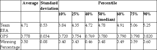 The results are as follows:
  = 0.94 - 0.100 × teamera,R2 = 0.49,SER = 0.06.
(0.08)(0.017)
= 0.94 - 0.100 × teamera,R2 = 0.49,SER = 0.06.
(0.08)(0.017)  = -0.68 + 1.513 × ops,R2=0.45,SER = 0.06.
(0.17)(0.221)
= -0.68 + 1.513 × ops,R2=0.45,SER = 0.06.
(0.17)(0.221)  = -0.19 - 0.099 × teamera + 1.490 × ops,R2=0.92,SER = 0.02.
(0.08)(0.008)(0.126)
(a)Use the t-statistic to test for the statistical significance of the coefficient.
(b)There are 30 teams in MLB.Does the small sample size worry you here when testing for significance?
= -0.19 - 0.099 × teamera + 1.490 × ops,R2=0.92,SER = 0.02.
(0.08)(0.008)(0.126)
(a)Use the t-statistic to test for the statistical significance of the coefficient.
(b)There are 30 teams in MLB.Does the small sample size worry you here when testing for significance?
(Essay)
4.7/5 (35)
Trying to remember the formula for the homoskedasticity-only F-statistic,you forgot whether you subtract the restricted SSR from the unrestricted SSR or the other way around.Your professor has provided you with a table containing critical values for the F distribution.How can this be of help?
(Essay)
4.8/5 (42)
When testing the null hypothesis that two regression slopes are zero simultaneously,then you cannot reject the null hypothesis at the 5% level,if the ellipse contains the point
(Multiple Choice)
4.8/5 (36)
Attendance at sports events depends on various factors.Teams typically do not change ticket prices from game to game to attract more spectators to less attractive games.However,there are other marketing tools used,such as fireworks,free hats,etc. ,for this purpose.You work as a consultant for a sports team,the Los Angeles Dodgers,to help them forecast attendance,so that they can potentially devise strategies for price discrimination.After collecting data over two years for every one of the 162 home games of the 2000 and 2001 season,you run the following regression:  = 15,005 + 201 × Temperat + 465 × DodgNetWin + 82 × OppNetWin
(8,770)(121)(169)(26)
+ 9647 × DFSaSu + 1328 × Drain + 1609 × D150m + 271 × DDiv - 978 × D2001;
(1505)(3355)(1819)(1,184)(1,143)
R2=0.416,SER = 6983
where Attend is announced stadium attendance,Temperat it the average temperature on game day,DodgNetWin are the net wins of the Dodgers before the game (wins-losses),OppNetWin is the opposing team's net wins at the end of the previous season,and DFSaSu,Drain,D150m,Ddiv,and D2001 are binary variables,taking a value of 1 if the game was played on a weekend,it rained during that day,the opposing team was within a 150 mile radius,the opposing team plays in the same division as the Dodgers,and the game was played during 2001,respectively.Numbers in parentheses are heteroskedasticity- robust standard errors.
(a)Are the slope coefficients statistically significant?
(b)To test whether the effect of the last four binary variables is significant,you have your regression program calculate the relevant F-statistic,which is 0.295.What is the critical value? What is your decision about excluding these variables?
= 15,005 + 201 × Temperat + 465 × DodgNetWin + 82 × OppNetWin
(8,770)(121)(169)(26)
+ 9647 × DFSaSu + 1328 × Drain + 1609 × D150m + 271 × DDiv - 978 × D2001;
(1505)(3355)(1819)(1,184)(1,143)
R2=0.416,SER = 6983
where Attend is announced stadium attendance,Temperat it the average temperature on game day,DodgNetWin are the net wins of the Dodgers before the game (wins-losses),OppNetWin is the opposing team's net wins at the end of the previous season,and DFSaSu,Drain,D150m,Ddiv,and D2001 are binary variables,taking a value of 1 if the game was played on a weekend,it rained during that day,the opposing team was within a 150 mile radius,the opposing team plays in the same division as the Dodgers,and the game was played during 2001,respectively.Numbers in parentheses are heteroskedasticity- robust standard errors.
(a)Are the slope coefficients statistically significant?
(b)To test whether the effect of the last four binary variables is significant,you have your regression program calculate the relevant F-statistic,which is 0.295.What is the critical value? What is your decision about excluding these variables?
(Essay)
4.9/5 (42)
Consider the following two models to explain testscores.
Model 1:
Dependent Variable: TESTSCR
Method: Least Squares
Date: 07/31/06 Time: 17:52
Sample: 1 420
Included observations: 420 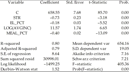 Model 2:
Dependent Variable: TESTSCR
Method: Least Squares
Date: 07/31/06 Time: 17:56
Sample: 1 420
Included observations: 420
Model 2:
Dependent Variable: TESTSCR
Method: Least Squares
Date: 07/31/06 Time: 17:56
Sample: 1 420
Included observations: 420 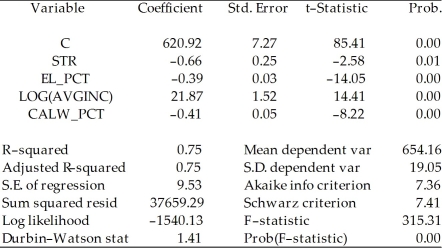 Explain why you cannot use the F-test in this situation to discriminate between Model 1 and Model 2.
(Essay)
4.7/5 (40)
Consider the following regression output for an unrestricted and a restricted model.
Unrestricted model:
Dependent Variable: TESTSCR
Method: Least Squares
Date: 07/31/06 Time: 17:35
Sample: 1 420
Included observations: 420  Restricted model:
Dependent Variable: TESTSCR
Method: Least Squares
Date: 07/31/06 Time: 17:37
Sample: 1 420
Included observations: 420
Restricted model:
Dependent Variable: TESTSCR
Method: Least Squares
Date: 07/31/06 Time: 17:37
Sample: 1 420
Included observations: 420  Calculate the homoskedasticity only F-statistic and determine whether the null hypothesis can be rejected at the 5% significance level.
(Essay)
4.7/5 (30)
All of the following are correct formulae for the homoskedasticity-only F-statistic,with the exception of
(Multiple Choice)
4.7/5 (29)
You are presented with the following output from a regression package,which reproduces the regression results of testscores on the student-teacher ratio from your textbook
Dependent Variable: TESTSCR
Method: Least Squares
Date: 07/30/06 Time: 17:44
Sample: 1 420
Included observations: 420 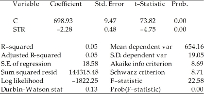 Std.Error are homoskedasticity only standard errors.
a)What is the relationship between the t-statistic on the student-teacher ratio coefficient and the F-statistic?
b)Next,two explanatory variables,the percent of English learners (EL_PCT)and expenditures per student (EXPN_STU)are added.The output is listed as below.What is the relationship between the three t-statistics for the slopes and the homoskedasticity-only F-statistic now?
Dependent Variable: TESTSCR
Method: Least Squares
Date: 07/30/06 Time: 17:55
Sample: 1 420
Included observations: 420
Std.Error are homoskedasticity only standard errors.
a)What is the relationship between the t-statistic on the student-teacher ratio coefficient and the F-statistic?
b)Next,two explanatory variables,the percent of English learners (EL_PCT)and expenditures per student (EXPN_STU)are added.The output is listed as below.What is the relationship between the three t-statistics for the slopes and the homoskedasticity-only F-statistic now?
Dependent Variable: TESTSCR
Method: Least Squares
Date: 07/30/06 Time: 17:55
Sample: 1 420
Included observations: 420 
(Essay)
4.9/5 (43)
Set up the null hypothesis and alternative hypothesis carefully for the following cases:
(a)k = 4,test for all coefficients other than the intercept to be zero
(b)k = 3,test for the slope coefficient of X1 to be unity,and the coefficients on the other explanatory variables to be zero
(c)k = 10,test for the slope coefficient of X1 to be zero,and for the slope coefficients of X2 and X3 to be the same but of opposite sign.
(d)k = 4,test for the slope coefficients to add up to unity
(Essay)
4.8/5 (40)
If you reject a joint null hypothesis using the F-test in a multiple hypothesis setting,then
(Multiple Choice)
4.8/5 (36)
The following linear hypothesis can be tested using the F-test with the exception of
(Multiple Choice)
4.8/5 (36)
In the multiple regression model,the t-statistic for testing that the slope is significantly different from zero is calculated
(Multiple Choice)
4.9/5 (33)
The F-statistic with q = 2 restrictions when testing for the restrictions β1 = 0 and β2 = 0 is given by the following formula:  Discuss how this formula can be understood intuitively.
(Essay)
4.9/5 (33)
All of the following are examples of joint hypotheses on multiple regression coefficients,with the exception of
(Multiple Choice)
5.0/5 (38)
Filters
- Essay(0)
- Multiple Choice(0)
- Short Answer(0)
- True False(0)
- Matching(0)