Exam 14: Introduction to Time Series Regression and Forecasting
Exam 1: Economic Questions and Data17 Questions
Exam 2: Review of Probability71 Questions
Exam 3: Review of Statistics63 Questions
Exam 4: Linear Regression With One Regressor65 Questions
Exam 5: Regression With a Single Regressor: Hypothesis Tests and Confidence Intervals59 Questions
Exam 6: Linear Regression With Multiple Regressors65 Questions
Exam 7: Hypothesis Tests and Confidence Intervals in Multiple Regression65 Questions
Exam 8: Nonlinear Regression Functions62 Questions
Exam 9: Assessing Studies Based on Multiple Regression65 Questions
Exam 10: Regression With Panel Data50 Questions
Exam 11: Regression With a Binary Dependent Variable50 Questions
Exam 12: Instrumental Variables Regression50 Questions
Exam 13: Experiments and Quasi-Experiments50 Questions
Exam 14: Introduction to Time Series Regression and Forecasting50 Questions
Exam 15: Estimation of Dynamic Causal Effects50 Questions
Exam 16: Additional Topics in Time Series Regression50 Questions
Exam 17: The Theory of Linear Regression With One Regressor49 Questions
Exam 18: The Theory of Multiple Regression50 Questions
Select questions type
Find data for real GDP (Yt)for the United States for the time period 1959:I (first quarter)to 1995:IV.Next generate two growth rates: The (annualized)quarterly growth rate of real GDP
[(lnYt - lnYt-1)× 400] and the annual growth rate of real GDP [(lnYt - lnYt-4)× 100].Which is more volatile? What is the reason for this? Explain.
Free
(Essay)
4.9/5  (39)
(39)
Correct Answer: Verified
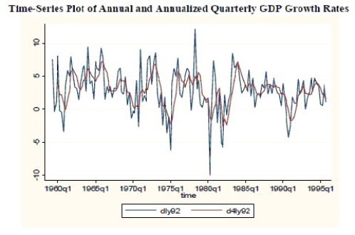 The quarterly growth rate that is more volatile because the annual growth rate is a moving average of the quarterly growth rate,and hence "wild swings" are smoothed out:
(lnYt - lnYt-4)= (lnYt - lnYt-1)+ (lnYt-1 - lnYt-2)+ (lnYt-2 - lnYt-3)+ (lnYt-3 - lnYt-4)
The Bayes-Schwarz Information Criterion (BIC)is given by the following formula
Free
(Multiple Choice)
4.9/5 (40)
Correct Answer:Verified
A
You want to determine whether or not the unemployment rate for the United States has a stochastic trend using the Augmented Dickey Fuller Test (ADF).The BIC suggests using 3 lags,while the AIC suggests 4 lags.
(a)Which of the two will you use for your choice of the optimal lag length?
(b)After estimating the appropriate equation,the t-statistic on the lag level unemployment rate is (-2.186)(using a constant,but not a trend).What is your decision regarding the stochastic trend of the unemployment rate series in the United States?
(c)Having worked in the previous exercise with the unemployment rate level,you repeat the exercise using the difference in United States unemployment rates.Write down the appropriate equation to conduct the Augmented Dickey-Fuller test here.The t-statistic on relevant coefficient turns out to be (-4.791).What is your conclusion now?
(Essay)
4.8/5 (35)
Negative autocorrelation in the change of a variable implies that
(Multiple Choice)
4.9/5 (40)
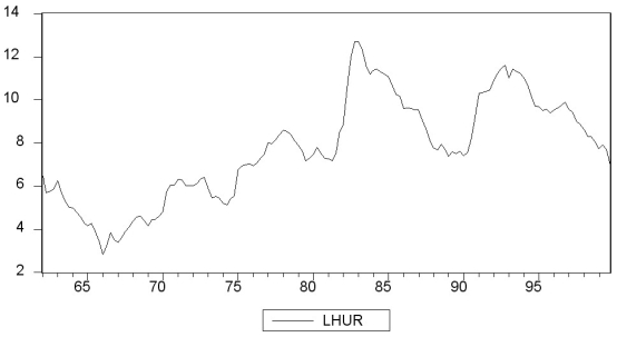
You have collected quarterly data on Canadian unemployment (UrateC)and inflation (InfC)from 1962 to 1999 with the aim to forecast Canadian inflation.
(a)To get a better feel for the data,you first inspect the plots for the series. 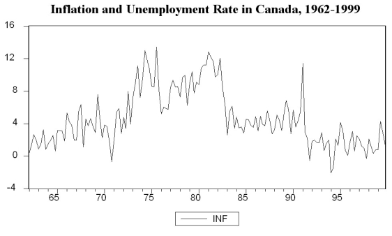
 Inspecting the Canadian inflation rate plot and having calculated the first autocorrelation to be 0.79 for the sample period,do you suspect that the Canadian inflation rate has a stochastic trend? What more formal methods do you have available to test for a unit root?
(b)You run the following regression,where the numbers in parenthesis are homoskedasticity-only standard errors:
Inspecting the Canadian inflation rate plot and having calculated the first autocorrelation to be 0.79 for the sample period,do you suspect that the Canadian inflation rate has a stochastic trend? What more formal methods do you have available to test for a unit root?
(b)You run the following regression,where the numbers in parenthesis are homoskedasticity-only standard errors:  = 0.49- 0.10 Inft-1 - 0.39 △InfCt-1 - 0.33 △InfCt-2 - 0.21 △InfCt-3 + 0.05 △InfCt-4
(0.28)(0.05)(0.09)(0.09)(0.09)(0.08)
Test for the presence of a stochastic trend.Should you have used heteroskedasticity-robust standard errors? Does the fact that you use quarterly data suggest including four lags in the above regression,or how should you determine the number of lags?
(c)To forecast the Canadian inflation rate for 2000:I,you estimate an AR(1),AR(4),and an ADL(4,1)model for the sample period 1962:I to 1999:IV.The results are as follows:
= 0.49- 0.10 Inft-1 - 0.39 △InfCt-1 - 0.33 △InfCt-2 - 0.21 △InfCt-3 + 0.05 △InfCt-4
(0.28)(0.05)(0.09)(0.09)(0.09)(0.08)
Test for the presence of a stochastic trend.Should you have used heteroskedasticity-robust standard errors? Does the fact that you use quarterly data suggest including four lags in the above regression,or how should you determine the number of lags?
(c)To forecast the Canadian inflation rate for 2000:I,you estimate an AR(1),AR(4),and an ADL(4,1)model for the sample period 1962:I to 1999:IV.The results are as follows:  = 0.002 - 0.31 △InfCt-1
(0.014)(0.10)
= 0.002 - 0.31 △InfCt-1
(0.014)(0.10)  = 0.021 - 0.46 ΔInfCt-1 - 0.39 ΔInfCt-2 - 0.25 ΔInfCt-3 + 0.03 ΔInfCt-4
(0.158)(0.10)(0.11)(0.08)(0.07)
= 0.021 - 0.46 ΔInfCt-1 - 0.39 ΔInfCt-2 - 0.25 ΔInfCt-3 + 0.03 ΔInfCt-4
(0.158)(0.10)(0.11)(0.08)(0.07)  = 1.279 - 0.51 ΔInfCt-1 - 0.44 ΔInfCt-2 - 0.30 ΔInfCt-3 - 0.02 ΔInfCt-4
(0.57)(0.10)(0.11)(0.09)(0.08)
- 0.16 UrateCt-1
(0.07)
In addition,you have the following information on inflation in Canada during the four quarters of 1999 and the first quarter of 2000:
Inflation and Unemployment in Canada,First Quarter 1999 to First Quarter 2000
= 1.279 - 0.51 ΔInfCt-1 - 0.44 ΔInfCt-2 - 0.30 ΔInfCt-3 - 0.02 ΔInfCt-4
(0.57)(0.10)(0.11)(0.09)(0.08)
- 0.16 UrateCt-1
(0.07)
In addition,you have the following information on inflation in Canada during the four quarters of 1999 and the first quarter of 2000:
Inflation and Unemployment in Canada,First Quarter 1999 to First Quarter 2000
 For each of the three models,calculate the predicted inflation rate for the period 2000:I and the forecast error.
(d)Perform a test on whether or not Canadian unemployment rates Granger-cause the Canadian inflation rate.
For each of the three models,calculate the predicted inflation rate for the period 2000:I and the forecast error.
(d)Perform a test on whether or not Canadian unemployment rates Granger-cause the Canadian inflation rate.
(Essay)
4.9/5 (40)
Pseudo out of sample forecasting can be used for the following reasons with the exception of
(Multiple Choice)
4.8/5 (38)
Statistical inference was a concept that was not too difficult to understand when using cross-sectional data.For example,it is obvious that a population mean is not the same as a sample mean (take weight of students at your college/university as an example).With a bit of thought,it also became clear that the sample mean had a distribution.This meant that there was uncertainty regarding the population mean given the sample information,and that you had to consider confidence intervals when making statements about the population mean.The same concept carried over into the two-dimensional analysis of a simple regression: knowing the height-weight relationship for a sample of students,for example,allowed you to make statements about the population height-weight relationship.In other words,it was easy to understand the relationship between a sample and a population in cross-sections.But what about time-series? Why should you be allowed to make statistical inference about some population,given a sample at hand (using quarterly data from 1962-2010,for example)? Write an essay explaining the relationship between a sample and a population when using time series.
(Essay)
4.9/5 (37)
You have decided to use the Dickey Fuller (DF)test on the United States aggregate unemployment rate (sample period 1962:I - 1995:IV).As a result,you estimate the following AR(1)model  t = 0.114 - 0.024 UrateUSt-1,R2 = 0.0118,SER = 0.3417
(0.121)(0.019)
You recall that your textbook mentioned that this form of the AR(1)is convenient because it allows for you to test for the presence of a unit root by using the t- statistic of the slope.Being adventurous,you decide to estimate the original form of the AR(1)instead,which results in the following output
t = 0.114 - 0.024 UrateUSt-1,R2 = 0.0118,SER = 0.3417
(0.121)(0.019)
You recall that your textbook mentioned that this form of the AR(1)is convenient because it allows for you to test for the presence of a unit root by using the t- statistic of the slope.Being adventurous,you decide to estimate the original form of the AR(1)instead,which results in the following output  t = 0.114 - 0.976 UrateUSt-1,R2 = 0.9510,SER = 0.3417
(0.121)(0.019)
You are surprised to find the constant,the standard errors of the two coefficients,and the SER unchanged,while the regression R2 increased substantially.Explain this increase in the regression R2.Why should you have been able to predict the change in the slope coefficient and the constancy of the standard errors of the two coefficients and the SER?
t = 0.114 - 0.976 UrateUSt-1,R2 = 0.9510,SER = 0.3417
(0.121)(0.019)
You are surprised to find the constant,the standard errors of the two coefficients,and the SER unchanged,while the regression R2 increased substantially.Explain this increase in the regression R2.Why should you have been able to predict the change in the slope coefficient and the constancy of the standard errors of the two coefficients and the SER?
(Essay)
4.8/5 (32)
The Akaike Information Criterion (AIC)is given by the following formula
(Multiple Choice)
4.7/5 (38)
(Requires Appendix material)Define the difference operator Δ = (1 - L)where L is the lag operator,such that LjYt = Yt-j.In general,  = (1- Lj)i,where i and j are typically omitted when they take the value of 1.Show the expressions in Y only when applying the difference operator to the following expressions,and give the resulting expression an economic interpretation,assuming that you are working with quarterly data:
(a)Δ4Yt
(b)
= (1- Lj)i,where i and j are typically omitted when they take the value of 1.Show the expressions in Y only when applying the difference operator to the following expressions,and give the resulting expression an economic interpretation,assuming that you are working with quarterly data:
(a)Δ4Yt
(b)  Yt
(c)
Yt
(c) 
 Yt
(d)
Yt
(d)  Yt
Yt
(Essay)
4.8/5 (47)
Consider the following model
Yt = α0 + α1  + ut
where the superscript "e" indicates expected values.This may represent an example where consumption depended on expected,or "permanent," income.Furthermore,let expected income be formed as follows:
+ ut
where the superscript "e" indicates expected values.This may represent an example where consumption depended on expected,or "permanent," income.Furthermore,let expected income be formed as follows:  =
=  + λ(Xt-1 -
  );0 < λ < 1
This particular type of expectation formation is called the "adaptive expectations hypothesis."
(a)In the above expectation formation hypothesis,expectations are formed at the beginning of the period,say the 1st of January if you had annual data.Give an intuitive explanation for this process.
(b)Transform the adaptive expectation hypothesis in such a way that the right hand side of the equation only contains observable variables,i.e. ,no expectations.
(c)Show that by substituting the resulting equation from the previous question into the original equation,you get an ADL(0,∞)type equation.How are the coefficients of the regressors related to each other?
(d)Can you think of a transformation of the ADL(0,∞)equation into an ADL(1,1)type equation,if you allowed the error term to be (ut - λut-1)?
);0 < λ < 1
This particular type of expectation formation is called the "adaptive expectations hypothesis."
(a)In the above expectation formation hypothesis,expectations are formed at the beginning of the period,say the 1st of January if you had annual data.Give an intuitive explanation for this process.
(b)Transform the adaptive expectation hypothesis in such a way that the right hand side of the equation only contains observable variables,i.e. ,no expectations.
(c)Show that by substituting the resulting equation from the previous question into the original equation,you get an ADL(0,∞)type equation.How are the coefficients of the regressors related to each other?
(d)Can you think of a transformation of the ADL(0,∞)equation into an ADL(1,1)type equation,if you allowed the error term to be (ut - λut-1)?
(Essay)
4.9/5 (39)
Consider the AR(1)model Yt = β0 + β1Yt-1 + ut,  < 1..
(a)Find the mean and variance of Yt.
(b)Find the first two autocovariances of Yt.
(c)Find the first two autocorrelations of Yt.
< 1..
(a)Find the mean and variance of Yt.
(b)Find the first two autocovariances of Yt.
(c)Find the first two autocorrelations of Yt.
(Essay)
4.9/5 (44)
To choose the number of lags in either an autoregression or in a time series regression model with multiple predictors,you can use any of the following test statistics with the exception of the
(Multiple Choice)
4.8/5 (38)
Filters
- Essay(0)
- Multiple Choice(0)
- Short Answer(0)
- True False(0)
- Matching(0)