Exam 10: Regression With Panel Data

The "before and after" specification,binary variable specification,and "entity-demeaned" specification produce identical OLS estimates

"Empirical studies of economic growth are flawed because many of the truly important underlying determinants,such as culture and institutions,are very hard to measure." Discuss this statement paying particular attention to simple cross-section data and panel data models.Use equations whenever possible to underscore your argument.

With Panel Data,regression software typically uses an "entity-demeaned" algorithm because

HAC standard errors and clustered standard errors are related as follows:

(Requires Appendix material)When the fifth assumption in the Fixed Effects regression (cov (uit,uis Xit,Xis)= 0 for t ≠ s)is violated,then

In the Fixed Effects regression model,you should exclude one of the binary variables for the entities when an intercept is present in the equation

When you add state fixed effects to a simple regression model for U.S.states over a certain time period,and the regression R2 increases significantly,then it is safe to assume that

In panel data,the regression error

In the panel regression analysis of beer taxes on traffic deaths,the estimation period is 1982-1988 for the 48 contiguous U.S.states.To test for the significance of time fixed effects,you should calculate the F-statistic and compare it to the critical value from your Fq,∞ distribution,which equals (at the 5% level)

In the panel regression analysis of beer taxes on traffic deaths,the estimation period is 1982-1988 for the 48 contiguous U.S.states.To test for the significance of time fixed effects,you should calculate the F-statistic and compare it to the critical value from your Fq,∞ distribution,where q equals

Consider estimating the effect of the beer tax on the fatality rate,using time and state fixed effect for the Northeast Region of the United States (Maine,Vermont,New Hampshire,Massachusetts,Connecticut and Rhode Island)for the period 1991-2001.If Beer Tax was the only explanatory variable,how many coefficients would you need to estimate,excluding the constant?

In the Fixed Effects regression model,using (n - 1)binary variables for the entities,the coefficient of the binary variable indicates

Your textbook modifies the four assumptions for the multiple regression model by adding a new assumption.This represents an extension of the cross-sectional data case,where errors are uncorrelated across entities.The new assumption requires the errors to be uncorrelated across time,conditional on the regressors as well (cov(uit,uis Xit,Xis)= 0 for t ≠ s. ). (a)Discuss why there might be correlation over time in the errors when you use U.S.state panel data.Does this mean that you should not use OLS as an estimator? (b)Now consider pairs of adjacent states such as Indiana and Michigan,Texas and Arkansas,New York and Connecticut,etc.Is it likely that the fifth assumption will hold here,even though the "contemporaneous" errors are correlated? If not,can you still use OLS for estimation?

Your textbook specifies a simple regression problem for two time periods for the years 1982 and 1988 as follows: FatalityRatei,1982 = β0 + β1BeerTaxi,1982 + ui,1982 FatalityRatei,1988 = β0 + β1BeerTaxi,1988 + ui,1988 After subtracting the first equation from the second equation,the authors estimate the model and find a negative intercept. a.Show how you would have to modify the two equations to allow for the presence of an intercept in the differenced model. b.What would the relative magnitude of the modified model have to be for you to find a negative intercept?

If you included both time and entity fixed effects in the regression model which includes a constant,then

In the panel regression analysis of beer taxes on traffic deaths,the estimation period is 1982-1988 for the 48 contiguous U.S.states.To test for the significance of entity fixed effects,you should calculate the F-statistic and compare it to the critical value from your Fq,∞ distribution,where q equals

The notation for panel data is (Xit,Yit),i = 1,... ,n and t = 1,... ,T because

Give at least three examples from macroeconomics and five from microeconomics that involve specified equations in a panel data analysis framework.Indicate in each case what the role of the entity and time fixed effects in terms of omitted variables might be.

You first encountered growth regression in your intermediate macroeconomics course ("beta-convergence regressions"),that is,conditionally on some initial condition in per capita income,different authors tried to find the determinants of growth.Since growth is a long-run phenomenon,various studies collected data for a panel of numerous countries using 10-year averages,over a time period stretching from 1960 to 2005.For example,a balanced panel might consist of 50 or so odd countries for the time periods 1960-1970,1971-1980,…,2000-2005.Instead of using two-way fixed effects (entity fixed effects and time fixed)authors often only employed time fixed effects.Why do you think that is? What sort of information would be lost if these authors employed entity fixed effects as well?

You learned in intermediate macroeconomics that certain macroeconomic growth models predict conditional convergence or a catch up effect in per capita GDP between the countries of the world.That is,countries which are further behind initially in per-capita GDP will grow faster than the leader.You gather data from the Penn World Tables to test this theory. (a)By limiting your sample to 24 OECD countries,you hope to have a more homogeneous set of countries in your sample,i.e. ,countries that are not too different with respect to their institutions.To simplify matters,you decide to only test for unconditional convergence.In that case,the laggards catch up even without taking into account differences in some of the driving variables.Your scatter plot and regression for the time period 1975-1989 are as follows: 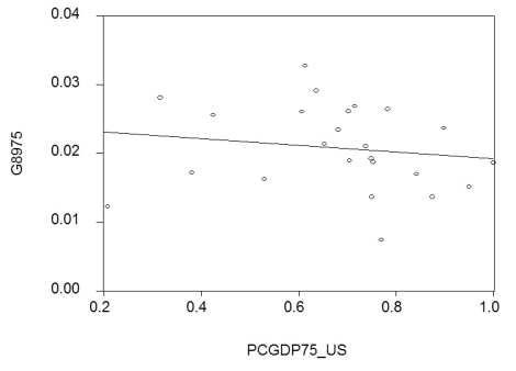= 0.024 - 0.005 PCGDP75_US;R2= 0.025,SER = 0.006 (0.06)(0.008) where is the average annual growth rate of per capita GDP from 1975-1989,and PCGDP75_US is per capita GDP relative to the United States in 1975.Numbers in parenthesis are heteroskedasticity-robust standard errors. Interpret the results.Is there indication of unconditional convergence? What critical value did you use? (b)Although you are quite discouraged by the result,you think that it might be due to the specific time period used.During this period,there were two OPEC oil price shocks with varying degrees of exposure for the OECD countries.You therefore repeat the exercise for the period 1960-1974,with the following results: 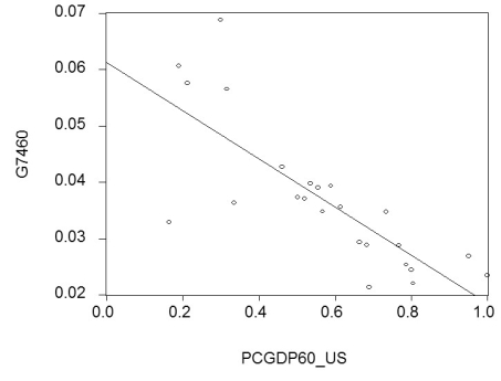= 0.061 - 0.043 PCGDP60_US;R2= 0.613,SER = 0.008 (0.004)(0.007) where is the average annual growth rate of per capita GDP from 1960-1974,and PCGDP60_US is per capita GDP relative to the United States in 1960. Compare this regression to the previous one. (c)You decide to run one more regression in differences.The dependent variable is now the change in the growth rate of per capita GDP from 1960-1974 to 1975-1989 (diffg)and the regressor the difference in the initial conditions (diffinit).This produces the following graph and regression: 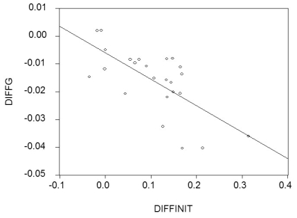= -0.006 - 0.096 × diffinit;R2 = 0.468;SER = 0.009 (0.03)(0.021) Interpret these results.Explain what has happened to unobservable omitted variables that are constant over time.Suggest what some of these variables might be. (d)Given that there are only two time periods,what other methods could you have employed to generate the identical results? Why do you think that the slope coefficient in this regression is significant given the results over the sub-periods?