Exam 17: Multiple Regression

Consider the following statistics of a multiple regression model: n = 25, k = 5, b ₁ = - 6.31, and s _e = 2.98. Can we conclude at the 1% significance level that x ₁ and y are linearly related?

In a multiple regression analysis, there are 20 data points and 4 independent variables, and the sum of the squared differences between observed and predicted values of y is 180. The standard error of estimate will be:

When an explanatory variable is dropped from a multiple regression model, the coefficient of determination can increase.

If a group of independent variables are not significant individually but are significant as a group at a specified level of significance, this is most likely due to:

In order to test the significance of a multiple regression model involving 4 independent variables and 25 observations, the numerator and denominator degrees of freedom for the critical value of F are 3 and 21, respectively.

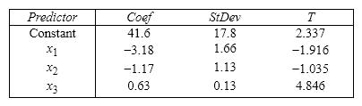
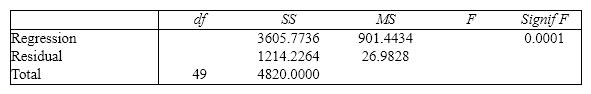
Student's Final Grade A statistics professor investigated some of the factors that affect an individual student's final grade in her course. She proposed the multiple regression model , where y   is the final grade (out of 100 points), x ₁ is the number of lectures skipped, x ₂ is the number of late assignments, and x ₃ is the midterm exam score (out of 100). The professor recorded the data for 50 randomly selected students. The computer output is shown below. 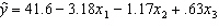THE REGRESSION EQUATION IS S = 13.74 R - Sq = 30.0% ANALYSIS OF VARIANCE 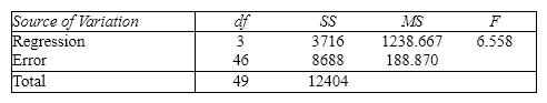{Student's Final Grade Narrative} Interpret the coefficient b ₂.

In a multiple regression analysis involving 4 independent variables and 30 data points, the number of degrees of freedom associated with the sum of squares for error, SSE, is 25.

The problem of multicollinearity arises when the:

A multiple regression model involves 40 observations and 4 independent variables produces a total variation in y of 100,000 and SSR = 80,400. Then, the value of MSE is 560.

In a multiple regression analysis, if the model provides a poor fit, this indicates that:

Suppose a multiple regression analysis involving 25 data points has and SSE = 36. Then, the number of the independent variables must be:

When the error variable does not have constant variance, this condition is called ____________________.

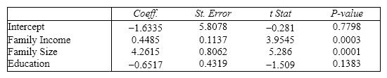
Life Expectancy An actuary wanted to develop a model to predict how long individuals will live. After consulting a number of physicians, she collected the age at death ( y ), the average number of hours of exercise per week ( x ₁), the cholesterol level ( x ₂), and the number of points that the individual's blood pressure exceeded the recommended value ( x ₃). A random sample of 40 individuals was selected. The computer output of the multiple regression model is shown below. THE REGRESSION EQUATION IS y = 55.8 + 1.79 x ₁ - 0.021 x ₂ - 0.061 x ₃ S = 9.47 R - Sq = 22.5% ANALYSIS OF VARIANCE {Life Expectancy Narrative} Is there enough evidence at the 1% significance level to infer that the average number of hours of exercise per week and the age at death are linearly related?

Real Estate Builder A real estate builder wishes to determine how house size is influenced by family income, family size, and education of the head of household. House size is measured in hundreds of square feet, income is measured in thousands of dollars, and education is measured in years. A partial computer output is shown below. SUMMARY OUTPUT 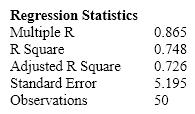ANOVA {Real Estate Builder Narrative} What minimum annual income would an individual with a family size of 4 and 16 years of education need to attain a predicted 10,000 square foot home?

Marc Anthony Concert At a recent Marc Anthony concert, a survey was conducted that asked a random sample of 20 people their age and how many concerts they have attended since the first of the year. The following data were collected: 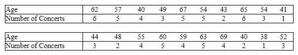An Excel output follows: 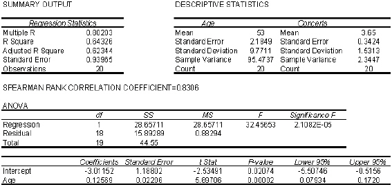{Marc Anthony Concert Narrative} Use the residuals to compute the standardized residuals.

How do you go about checking for multicollinearity?

Life Expectancy An actuary wanted to develop a model to predict how long individuals will live. After consulting a number of physicians, she collected the age at death ( y ), the average number of hours of exercise per week ( x ₁), the cholesterol level ( x ₂), and the number of points that the individual's blood pressure exceeded the recommended value ( x ₃). A random sample of 40 individuals was selected. The computer output of the multiple regression model is shown below. THE REGRESSION EQUATION IS y = 55.8 + 1.79 x ₁ - 0.021 x ₂ - 0.061 x ₃ 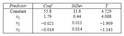S = 9.47 R - Sq = 22.5% ANALYSIS OF VARIANCE 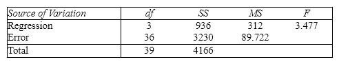{Life Expectancy Narrative} Is there enough evidence at the 5% significance level to infer that the model is useful in predicting length of life?

Multicollinearity is present if the dependent variable is linearly related to one of the explanatory variables.

One of the consequences of multicollinearity in multiple regression is biased estimates on the slope coefficients.

Some of the requirements for the error variable in a multiple regression model are that the standard deviation is a(n)____________________ and the errors are ____________________.