Exam 7: Hypothesis Tests and Confidence Intervals in Multiple Regression

You have estimated the following regression to explain hourly wages,using a sample of 250 individuals: AHEi = -2.44 - 1.57 × DFemme + 0.27 × DMarried + 0.59 × Educ + 0.04 × Exper - 0.60 × DNonwhite (1.29)(0.33)(0.36)(0.09)(0.01)(0.49) + 0.13 × NCentral - 0.11 × South (0.59)(0.58) R2 = 0.36,SER = 2.74,n = 250 Numbers in parenthesis are heteroskedasticity robust standard errors.Add "*"(5%)and "**" (1%)to indicate statistical significance of the coefficients.

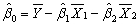
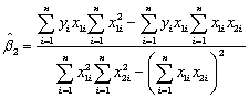
In the multiple regression model with two explanatory variables Yi = β0 + β1X1i + β2X2i + ui the OLS estimators for the three parameters are as follows (small letters refer to deviations from means as in zi = Zi - ): You have collected data for 104 countries of the world from the Penn World Tables and want to estimate the effect of the population growth rate (X1i)and the saving rate (X2i)(average investment share of GDP from 1980 to 1990)on GDP per worker (relative to the U.S. )in 1990.The various sums needed to calculate the OLS estimates are given below: = 33.33; = 2.025; =17.313 = 8.3103; = .0122; = 0.6422 = - 0.2304; = 1.5676; = -0.0520 The heteroskedasticity-robust standard errors of the two slope coefficients are 1.99 (for population growth)and 0.23 (for the saving rate).Calculate the 95% confidence interval for both coefficients.How many standard deviations are the coefficients away from zero?

The cost of attending your college has once again gone up.Although you have been told that education is investment in human capital,which carries a return of roughly 10% a year,you (and your parents)are not pleased.One of the administrators at your university/college does not make the situation better by telling you that you pay more because the reputation of your institution is better than that of others.To investigate this hypothesis,you collect data randomly for 100 national universities and liberal arts colleges from the 2000-2001 U.S.News and World Report annual rankings.Next you perform the following regression = 7,311.17 + 3,985.20 × Reputation - 0.20 × Size (2,058.63)(664.58)(0.13) + 8,406.79 × Dpriv - 416.38 × Dlibart - 2,376.51 × Dreligion (2,154.85)(1,121.92)(1,007.86) R2=0.72,SER = 3,773.35 where Cost is Tuition,Fees,Room and Board in dollars,Reputation is the index used in U.S.News and World Report (based on a survey of university presidents and chief academic officers),which ranges from 1 ("marginal")to 5 ("distinguished"),Size is the number of undergraduate students,and Dpriv,Dlibart,and Dreligion are binary variables indicating whether the institution is private,a liberal arts college,and has a religious affiliation.The numbers in parentheses are heteroskedasticity-robust standard errors. (a)Indicate whether or not the coefficients are significantly different from zero. (b)What is the p-value for the null hypothesis that the coefficient on Size is equal to zero? Based on this,should you eliminate the variable from the regression? Why or why not? (c)You want to test simultaneously the hypotheses that βsize = 0 and βDilbert = 0.Your regression package returns the F-statistic of 1.23.Can you reject the null hypothesis? (d)Eliminating the Size and Dlibart variables from your regression,the estimation regression becomes = 5,450.35 + 3,538.84 × Reputation + 10,935.70 × Dpriv - 2,783.31 × Dreligion; (1,772.35)(590.49)(875.51)(1,180.57) R2=0.72,SER = 3,792.68 Why do you think that the effect of attending a private institution has increased now? (e)You give a final attempt to bring the effect of Size back into the equation by forcing the assumption of homoskedasticity onto your estimation.The results are as follows: = 7,311.17 + 3,985.20 × Reputation - 0.20 × Size (1,985.17)(593.65)(0.07) + 8,406.79 × Dpriv - 416.38 × Dlibart - 2,376.51 × Dreligion (1,423.59)(1,096.49)(989.23) R2=0.72,SER = 3,682.02 Calculate the t-statistic on the Size coefficient and perform the hypothesis test that its coefficient is zero.Is this test reliable? Explain.

Analyzing a regression using data from a sub-sample of the Current Population Survey with about 4,000 observations,you realize that the regression R2,and the adjusted R2, 2,are almost identical.Why is that the case? In your textbook,you were told that the regression R2 will almost always increase when you add an explanatory variable,but that the adjusted measure does not have to increase with such an addition.Can this still be true?

The confidence interval for a single coefficient in a multiple regression

Prove that

The OLS estimators of the coefficients in multiple regression will have omitted variable bias

Consider a situation where economic theory suggests that you impose certain restrictions on your estimated multiple regression function.These may involve the equality of parameters,such as the returns to education and on the job training in earnings functions,or the sum of coefficients,such as constant returns to scale in a production function.To test the validity of your restrictions,you have your statistical package calculate the corresponding F-statistic.Find the critical value from the F-distribution at the 5% and 1% level,and comment whether or not you will reject the null hypothesis in each of the following cases. (a)number of observations: 152;number of restrictions: 3;F-statistic: 3.21 (b)number of observations: 1,732;number of restrictions:7;F-statistic: 4.92 (c)number of observations: 63;number of restrictions: 1;F-statistic: 2.47 (d)number of observations: 4,000;number of restrictions: 5;F-statistic: 1.82 (e)Explain why you can use the Fq,∞ distribution to compute the critical values in (a)-(d).

The homoskedasticity only F-statistic is given by the formula where SSRrestricted is the sum of squared residuals from the restricted regression,SSRunrestricted is the sum of squared residuals from the unrestricted regression,q is the number of restrictions under the null hypothesis,and kunrestricted is the number of regressors in the unrestricted regression.Prove that this formula is the same as the following formula based on the regression R2 of the restricted and unrestricted regression:

Using the California School data set from your textbook,you decide to run a regression of the average reading score (ScrRead)on the average mathematics score (ScrMaths).The result is as follows,where the numbers in parenthesis are homoskedasticity only standard errors: = 8.47 + 0.9895×ScrMaths (13.20)(0.0202) N = 420,R2 = 0.85,SER = 7.8 You believe that the average mathematics score is an unbiased predictor of the average reading score.Consider the above regression to be the unrestricted from which you would calculate SSRUnrestricted .How would you find the SSRRestricted? How many restrictions would have to impose?

Consider the regression output from the following unrestricted model: Unrestricted model: Dependent Variable: TESTSCR Method: Least Squares Date: 07/31/06 Time: 17:35 Sample: 1 420 Included observations: 420 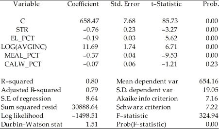To test for the null hypothesis that neither coefficient on the percent eligible for subsidized lunch nor the coefficient on the percent on public income assistance is statistically significant,you have your statistical package plot the confidence set.Interpret the graph below and explain what it tells you about the null hypothesis.

Looking at formula (7.13)in your textbook for the homoskedasticity-only F-statistic, 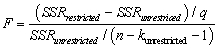give three conditions under which,ceteris paribus,you would find a large value,and hence would be likely to reject the null hypothesis.

The formula for the standard error of the regression coefficient,when moving from one explanatory variable to two explanatory variables,

Consider the following regression using the California School data set from your textbook. = 681.44 - 0.61LchPct n=420,R2=0.75,SER=9.45 where TestScore is the test score and LchPct is the percent of students eligible for subsidized lunch (average = 44.7,max = 100,min = 0). a.What is the effect of a 20 percentage point increase in the student eligible for subsidized lunch? b.Your textbook started with the following regression in Chapter 4: = 698.9 - 2.28STR n=420,R2=0.051,SER=18.58 where STR is the student teacher ratio. Your textbook tells you that in the multiple regression framework considered,the percentage of students eligible for subsidized lunch is a control variable,while the student teacher ratio is the variable of interest.Given that the regression R2 is so much higher for the first equation than for the second equation,shouldn't the role of the two variables be reversed? That is,shouldn't the student teacher ratio be the control variable while the percent of students eligible for subsidized lunch be the variable of interest?

Adding the Percent of English Speakers (PctEL)to the Student Teacher Ratio (STR)in your textbook reduced the coefficient for STR from 2.28 to 1.10 with a standard error of 0.43.Construct a 90% and 99% confidence interval to test the hypothesis that the coefficient of STR is 2.28.

You have estimated the following regression to explain hourly wages,using a sample of 250 individuals: = -2.44 - 1.57 × DFemme + 0.27 × DMarried + 0.59 × Educ + 0.04 × Exper - 0.60 × DNonwhite (1.29)(0.33)(0.36)(0.09)(0.01)(0.49) + 0.13 × NCentral - 0.11 × South (0.59)(0.58) R2 = 0.36,SER = 2.74,n = 250 Test the null hypothesis that the coefficients on DMarried,DNonwhite,and the two regional variables,NCentral and South are zero.The F-statistic for the null hypothesis βmarried = βnonwhite = βnonwhite = βncentral = βsouth = 0 is 0.61.Do you reject the null hypothesis?

You have collected data for 104 countries to address the difficult questions of the determinants for differences in the standard of living among the countries of the world.You recall from your macroeconomics lectures that the neoclassical growth model suggests that output per worker (per capita income)levels are determined by,among others,the saving rate and population growth rate.To test the predictions of this growth model,you run the following regression: = 0.339 - 12.894 × n + 1.397 × SK,R2=0.621,SER = 0.177 (0.068)(3.177)(0.229) where RelPersInc is GDP per worker relative to the United States,n is the average population growth rate,1980-1990,and SK is the average investment share of GDP from 1960 to 1990 (remember investment equals saving).Numbers in parentheses are for heteroskedasticity-robust standard errors. (a)Calculate the t-statistics and test whether or not each of the population parameters are significantly different from zero. (b)The overall F-statistic for the regression is 79.11.What is the critical value at the 5% and 1% level? What is your decision on the null hypothesis? (c)You remember that human capital in addition to physical capital also plays a role in determining the standard of living of a country.You therefore collect additional data on the average educational attainment in years for 1985,and add this variable (Educ)to the above regression.This results in the modified regression output: = 0.046 - 5.869 × n + 0.738 × SK + 0.055 × Educ,R2=0.775,SER = 0.1377 (0.079)(2.238)(0.294)(0.010) How has the inclusion of Educ affected your previous results? (d)Upon checking the regression output,you realize that there are only 86 observations,since data for Educ is not available for all 104 countries in your sample.Do you have to modify some of your statements in (d)?

At a mathematical level,if the two conditions for omitted variable bias are satisfied,then

Consider a regression with two variables,in which X1i is the variable of interest and X2i is the control variable.Conditional mean independence requires

To calculate the homoskedasticity-only overall regression F-statistic,you need to compare the SSRrestricted with the SSRunrestricted.Consider the following output from a regression package,which reproduces the regression results of testscores on the student-teacher ratio,the percent of English learners,and the expenditures per student from your textbook: Dependent Variable: TESTSCR Method: Least Squares Date: 07/30/06 Time: 17:55 Sample: 1 420 Included observations: 420 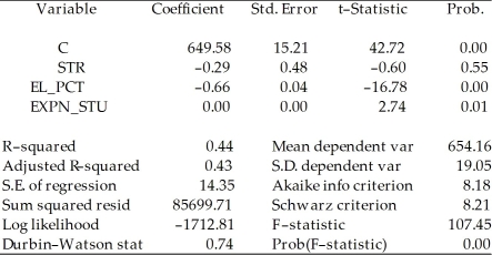Sum of squared resid corresponds to SSRunrestricted.How are you going to find SSRrestricted?