Exam 15: Introduction to Simulation Modeling

A discrete distribution is useful for many situations, either when the uncertain quantity is not continuous (the number of televisions demanded, for example) or when we want a discrete approximation to a continuous variable.

A company is about to develop and then market a new product. It wants to build a simulation model for the entire process, and one key uncertain input is the development cost. For each of the scenarios in the questions below, choose an "appropriate" distribution, together with its parameters, and explain your choice. -(A) Company experts have no idea about the distribution of their development cost. All they can state is that "we are 90% sure it will be somewhere between $450,000 and $650,000." ​ (B) Company experts can still make the same two statements as in (A), but now they can also state that "we believe the distribution is symmetric and its most likely value is about $550,000." ​ (C) Company experts can still make the same two statements as in (A), but now they can also state that "we believe the distribution is skewed to the right, and its most likely value is about $500,000."

(A) What are the appropriate probability distributions to model the number of faculty members showing up in each lot? (B) Given the current situation, estimate the probability that on a peak day, at least one faculty member with a sticker will be unable to find a parking space. Assume that the number who shows up at each lot is independent of the number who shows up at the other two lots. (C) Suppose that faculty members are allowed to park in any lot. Does this help solve the problem? Why or why not? (D) Suppose that the numbers of faculty who show up at the three lots are correlated, with each correlation equal to 0.80. Does your answer to (C) change? Why or why not?

One of the primary advantages of simulation models is that they enable managers to answer what-if questions about changes in systems without actually changing the systems themselves.

If you add several normally distributed random numbers, the result is normally distributed, where the mean of the sum is the sum of the individual means, and the variance of the sum is the sum of the individual variances. This result is difficult to prove mathematically, but it is easy to demonstrate with simulation. To do so, run a simulation where you add three normally distributed random numbers, each with mean 100 and standard deviation 10. Your single output variable should be the sum of these three numbers. Verify with @RISK that the distribution of this output is approximately normal with mean 300 and variance 300 (hence, standard deviation = 17.32).

The normal distribution is often used in simulation models because it is the most common distribution in statistics and it does not allow negative values.

Suppose you are going to invest equal amounts in three stocks. The annual return from each stock is normally distributed with a mean of 0.01 (1%) and a standard deviation of 0.06. The annual return on your portfolio, the output variable of interest, is the average of the three stock returns. Run @RISK, using 1000 iterations, on each of the scenarios described in the questions below, and report few results from the summary report sheets. -(A) The three stock returns are highly correlated. The correlation between each pair is 0.9 (B) The three stock returns are practically independent. The correlation between each pair is 0.1 (C) The first two stocks are moderately correlated. The correlation between their returns is 0.4. The third stock's return is negatively correlated with the other two. The correlation between its return and each of the first two is -0.8. (D) Compare the portfolio distributions from @RISK for the three scenarios in (A), (B) and (C). What do you conclude? (E) You might think of a fourth scenario, where the correlation between each pair of returns is a large negative number such as -0.80. But explain intuitively why this makes no sense. Try running a simulation with these negative correlations to see what happens.

Correlation between two random input variables might not change the mean of an output, but it can definitely affect the variability and shape of an output distribution.

Which of the following statements are false regarding the numbers generated by the RAND function in Excel^®?

A company is about to develop and then market a new product. It wants to build a simulation model for the entire process, and one key uncertain input is the development time, which is measured in an integer number of months. For each of the scenarios in the questions below, choose an "appropriate" distribution, together with its parameters, and explain your choice. -Company experts believe the development time will fall into the range of 5 to 9 months. They believe the probabilities of the extremes (5 and 9 months) are both 10%, and the probabilities will vary linearly from those endpoints to a most likely value at 7 months.

The "random" numbers generated by the RAND function (or by any other package's random number generator) are not really random.

Each different set of values obtained for the uncertain quantities in a simulation model can considered to be:

A primary difference between standard spreadsheet models and simulation models is that at least one of the input variable cells in a simulation model contains random numbers.

Oregon State University has reached the final four in the 2016 NCAA Women's Basketball Tournament, and as a result, a sweatshirt supplier in Corvallis is trying to decide how many sweatshirts to print for the upcoming championships. The final four teams (Oregon State, University of Washington, Syracuse, and University of Connecticut) have emerged from the quarterfinal round, and there is a week left until the semifinals, which are then followed in a couple of days by the finals. Each sweatshirt costs $12 to produce and sells for $24. However, in three weeks, any leftover sweatshirts will be put on sale for half price, $12. The supplier assumes that the demand (in thousands) for his sweatshirts during the next three weeks, when interest is at its highest, follows the probability distribution shown in the table below. The residual demand, after the sweatshirts have been put on sale, also has the probability distribution shown in the table below. The supplier realizes that every sweatshirt sold, even at the sale price, yields a profit. However, he also realizes that any sweatshirts produced but not sold must be thrown away, resulting in a $12 loss per sweatshirt. ​ Demand distribution at regular price Demand distribution at reduced price ​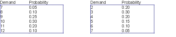 -Use @RISK simulation add-in to analyze the sweatshirt sales. Do this for normal distributions, where we assume that the regular demand is normally distributed with mean 10,000 and standard deviation 1500, and that the demand at the reduced price is normally distributed with mean 5,000 and standard deviation 1500.

A company is about to develop and then market a new product. It wants to build a simulation model for the entire process, and one key uncertain input is the development time, which is measured in an integer number of months. For each of the scenarios in the questions below, choose an "appropriate" distribution, together with its parameters, and explain your choice. -Company experts believe the development time will be from 5 to 9 months, but they have absolutely no idea which of these will result.

Many companies have used simulation to determine which of several possible investment projects they should choose. This is often referred to as

The flaw of averages is the reason deterministic models can be very misleading.

When we maximize or minimize the value of a decision variable by running several simulations simultaneously, we have found an optimal solution to the problem and attitude toward risk becomes irrelevant.

If we want to model a random stock price, we should do so with an unbounded symmetric probability distribution.

Oregon State University has reached the final four in the 2016 NCAA Women's Basketball Tournament, and as a result, a sweatshirt supplier in Corvallis is trying to decide how many sweatshirts to print for the upcoming championships. The final four teams (Oregon State, University of Washington, Syracuse, and University of Connecticut) have emerged from the quarterfinal round, and there is a week left until the semifinals, which are then followed in a couple of days by the finals. Each sweatshirt costs $12 to produce and sells for $24. However, in three weeks, any leftover sweatshirts will be put on sale for half price, $12. The supplier assumes that the demand (in thousands) for his sweatshirts during the next three weeks, when interest is at its highest, follows the probability distribution shown in the table below. The residual demand, after the sweatshirts have been put on sale, also has the probability distribution shown in the table below. The supplier realizes that every sweatshirt sold, even at the sale price, yields a profit. However, he also realizes that any sweatshirts produced but not sold must be thrown away, resulting in a $12 loss per sweatshirt. ​ Demand distribution at regular price Demand distribution at reduced price ​ -(A) Assume that the weight of each can in a six-pack has a 0.8 correlation with the weight of the other cans in the six-pack. What mean fill quantity (within 0.05 ounce) maximizes expected profit per six-pack? ​ (B) If the weights of the cans in the six-pack are probabilistically independent, what mean fill quantity (within 0.05 ounce) will maximize expected profit per six-pack? ​ (C) How can you explain the difference in the answers for (A) and (B)?