Exam 5: Regression With a Single Regressor: Hypothesis Tests and Confidence Intervals

You recall from one of your earlier lectures in macroeconomics that the per capita income depends on the savings rate of the country: those who save more end up with a higher standard of living.To test this theory,you collect data from the Penn World Tables on GDP per worker relative to the United States (RelProd)in 1990 and the average investment share of GDP from 1980-1990 (SK),remembering that investment equals saving.The regression results in the following output: = -0.08 + 2.44×SK,R2=0.46,SER = 0.21 (0.04)(0.38) (a)Interpret the regression results carefully. (b)Calculate the t-statistics to determine whether the two coefficients are significantly different from zero.Justify the use of a one-sided or two-sided test. (c)You accidentally forget to use the heteroskedasticity-robust standard errors option in your regression package and estimate the equation using homoskedasticity-only standard errors.This changes the results as follows: = -0.08 + 2.44×SK,R2=0.46,SER = 0.21 (0.04)(0.26) You are delighted to find that the coefficients have not changed at all and that your results have become even more significant.Why haven't the coefficients changed? Are the results really more significant? Explain. (d)Upon reflection you think about the advantages of OLS with and without homoskedasticity-only standard errors.What are these advantages? Is it likely that the error terms would be heteroskedastic in this situation?

Assume that your population regression function is Yi = βiXi + ui i.e. ,a regression through the origin (no intercept).Under the homoskedastic normal regression assumptions,the t-statistic will have a Student t distribution with n-1 degrees of freedom,not n-2 degrees of freedom,as was the case in Chapter 5 of your textbook.Explain.Do you think that the residuals will still sum to zero for this case?

Using data from the Current Population Survey,you estimate the following relationship between average hourly earnings (ahe)and the number of years of education (educ): = -4.58 + 1.71 educ The heteroskedasticity-robust standard error on the slope is (0.03).Calculate the 95% confidence interval for the slope.Repeat the exercise using the 90% and then the 99% confidence interval.Can you reject the null hypothesis that the slope coefficient is zero in the population?

Your textbook discussed the regression model when X is a binary variable Yi = β0 + βiDi + ui,i = 1,... ,n Let Y represent wages,and let D be one for females,and 0 for males.Using the OLS formula for the intercept coefficient,prove that is the average wage for males.

The only difference between a one- and two-sided hypothesis test is

In many of the cases discussed in your textbook,you test for the significance of the slope at the 5% level.What is the size of the test? What is the power of the test? Why is the probability of committing a Type II error so large here?

Explain carefully the relationship between a confidence interval,a one-sided hypothesis test,and a two-sided hypothesis test.What is the unit of measurement of the t-statistic?

Using 143 observations,assume that you had estimated a simple regression function and that your estimate for the slope was 0.04,with a standard error of 0.01.You want to test whether or not the estimate is statistically significant.Which of the following possible decisions is the only correct one:

(Requires Appendix)(Continuation from Chapter 4)At a recent county fair,you observed that at one stand people's weight was forecasted,and were surprised by the accuracy (within a range).Thinking about how the person could have predicted your weight fairly accurately (despite the fact that she did not know about your "heavy bones"),you think about how this could have been accomplished.You remember that medical charts for children contain 5%,25%,50%,75% and 95% lines for a weight/height relationship and decide to conduct an experiment with 110 of your peers.You collect the data and calculate the following sums: where the height is measured in inches and weight in pounds.(Small letters refer to deviations from means as in zi = Zi - . ) (a)Calculate the homoskedasticity-only standard errors and,using the resulting t-statistic,perform a test on the null hypothesis that there is no relationship between height and weight in the population of college students. (b)What is the alternative hypothesis in the above test,and what level of significance did you choose? (c)Statistics and econometrics textbooks often ask you to calculate critical values based on some level of significance,say 1%,5%,or 10%.What sort of criteria do you think should play a role in determining which level of significance to choose? (d)What do you think the relationship is between testing for the significance of the slope and whether or not the regression R2 is zero?

The homoskedastic normal regression assumptions are all of the following with the exception of:

With heteroskedastic errors,the weighted least squares estimator is BLUE.You should use OLS with heteroskedasticity-robust standard errors because

Consider the following two models involving binary variables as explanatory variables: = + DFemme and = DFemme + Male where Wage is the hourly wage rate,DFemme is a binary variable that is equal to 1 if the person is a female,and 0 if the person is a male.Male = 1 - DFemme.Even though you have not learned about regression functions with two explanatory variables (or regressions without an intercept),assume that you had estimated both models,i.e. ,you obtained the estimates for the regression coefficients. What is the predicted wage for a male in the two models? What is the predicted wage for a female in the two models? What is the relationship between the β s and the φs? Why would you prefer one model over the other?

If the absolute value of your calculated t-statistic exceeds the critical value from the standard normal distribution,you can

Under the least squares assumptions (zero conditional mean for the error term,Xi and Yi being i.i.d. ,and Xi and ui having finite fourth moments),the OLS estimator for the slope and intercept

A binary variable is often called a

Changing the units of measurement obviously will have an effect on the slope of your regression function.For example,let Y*= aY and X* = bX.Then it is easy but tedious to show that 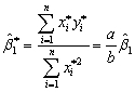.Given this result,how do you think the standard errors and the regression R2 will change?

The confidence interval for the sample regression function slope

In a Monte Carlo study,econometricians generate multiple sample regression functions from a known population regression function.For example,the population regression function could be Yi = β0 + β1Xi = 100 - 0.5 Xi.The Xs could be generated randomly or,for simplicity,be nonrandom ("fixed over repeated samples").If we had ten of these Xs,say,and generated twenty Ys,we would obviously always have all observations on a straight line,and the least squares formulae would always return values of 100 and 0.5 numerically.However,if we added an error term,where the errors would be drawn randomly from a normal distribution,say,then the OLS formulae would give us estimates that differed from the population regression function values.Assume you did just that and recorded the values for the slope and the intercept.Then you did the same experiment again (each one of these is called a "replication").And so forth.After 1,000 replications,you plot the 1,000 intercepts and slopes,and list their summary statistics. Sample: 1 1000 BETA0_HAT BETA1_HAT Mean 100.014 -0.500 Median 100.021 -0.500 Maximum 106.348 -0.468 Minimum 93.862 -0.538 Std.Dev.1.994 0.011 Skewness 0.013 -0.042 Kurtosis 3.026 2.986 Jarque-Bera 0.055 0.305 Probability 0.973 0.858 Sum 100014.353 -499.857 Sum Sq.Dev.3972.403 0.118 Observations 1000.000 1000.000 Here are the corresponding graphs: 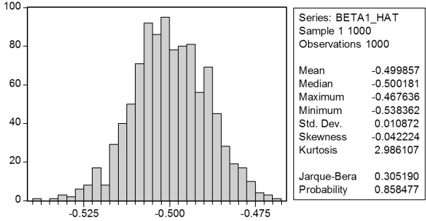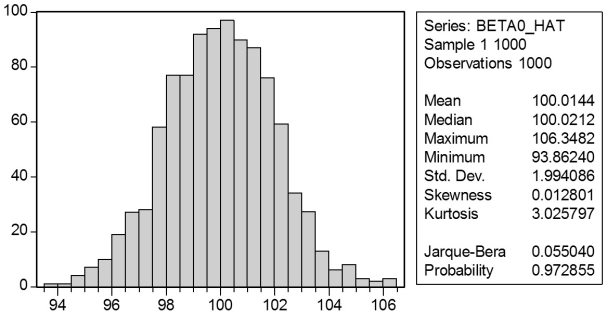Using the means listed next to the graphs,you see that the averages are not exactly 100 and -0.5.However,they are "close." Test for the difference of these averages from the population values to be statistically significant.

Finding a small value of the p-value (e.g.less than 5%)

When estimating a demand function for a good where quantity demanded is a linear function of the price,you should