Exam 4: Describing the Relation Between Two Variables
Exam 1: Data Collection34 Questions
Exam 2: Organizing and Summarizing Data30 Questions
Exam 3: Numerically Summarizing Data66 Questions
Exam 4: Describing the Relation Between Two Variables92 Questions
Exam 5: Probability91 Questions
Exam 6: Discrete Probability Distributions32 Questions
Exam 7: The Normal Probability Distributions36 Questions
Exam 8: Sampling Distributions12 Questions
Exam 9: Estimating the Value of a Parameter Using Confidence Intervals24 Questions
Exam 10: Hypothesis Tests Regarding a Parameter36 Questions
Exam 11: Inference on Two Samples65 Questions
Exam 12: Inference on Categorical Data16 Questions
Exam 13: Comparing Three or More Means15 Questions
Exam 14: Inference of the Least-Squares Regression Model28 Questions
Select questions type
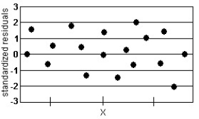
Analyze the residual lot below. Does it violate any of the conditions for an adequate linear model?
-
(Multiple Choice)
4.8/5  (26)
(26)
Compute the linear correlation coefficient between the two variables and determine whether a linear relation exists.
-
(Multiple Choice)
4.9/5 (37)
A county real estate appraiser wants to develop a statistical model to predict the appraised value of houses in a section of the county called East Meadow. One of the many variables thought to be an important predictor of appraised value is the number of rooms in the house. Consequently, the appraiser decided to fit the simple linear regression model,  where y = appraised value of the house (in $thousands) and x = number of rooms. Using data collected for a sample of n= 74 houses in East Meadow, the following results were obtained:
 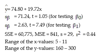 Give a practical interpretation of the estimate of the y-intercept of the least squares line.
(Multiple Choice)
4.7/5 (37)
The data below show the age and favorite type of music of 779 randomly selected people. Use  What, if any, association exists between favorite music and age? Discuss the association.
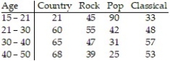
(Essay)
5.0/5 (40)
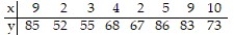
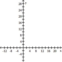
Construct a scatter diagram for the data.
-The scores of nine members of a local community college women's golf team in two rounds of tournament play are listed below. 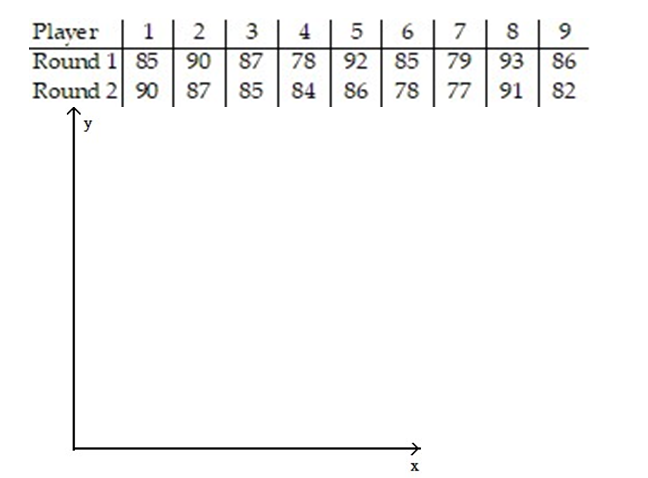
(Essay)
4.9/5 (36)
In an area of Russia, records were kept on the relationship between the rainfall (in inches) and the yield of wheat (bushels per acre). The data for a 9 year period is as follows:  The equation of the line of least squares is given as
  = -9.12 + 4.38x.
- How many bushels of wheat per acre can be predicted if it is expected that there will be 30 inches of rain?
= -9.12 + 4.38x.
- How many bushels of wheat per acre can be predicted if it is expected that there will be 30 inches of rain?
(Multiple Choice)
4.8/5 (32)
Is there a relationship between the raises administrators at State University receive and their performance on the job? A faculty group wants to determine whether job rating (x) is a useful linear predictor of raise (y). Consequently, the group considered the straight-line regression model,  Using the method of least squares, the faculty group obtained the following prediction equation,
  Interpret the estimated slope of the line.
(Multiple Choice)
4.9/5 (46)
Civil engineers often use the straight-line equation, E(y) =  +
+  x, to model the relationship between the mean shear strength E(y) of masonry joints and precompression stress, x. To test this theory, a series of stress tests were performed on solid bricks arranged in triplets and joined with mortar. The precompression stress was varied for each triplet and the ultimate shear load just before failure (called the shear strength) was recorded. The stress results for n = 7 triplet tests is shown in the accompanying table followed by a SAS printout of the regression analysis.
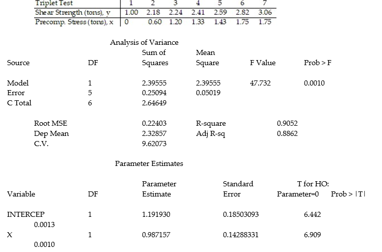
(Multiple Choice)
4.8/5 (33)
Use the linear correlation coefficient given to determine the coefficient of determination ,  -r = -0.42
(Multiple Choice)
4.8/5 (29)
Is there a relationship between the raises administrators at State University receive and their performance on the job? A faculty group wants to determine whether job rating (x) is a useful linear predictor of raise (y). Consequently, the group considered the straight-line regression model,  Using the method of least squares, the faculty group obtained the following prediction equation,
 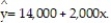 Interpret the estimated y-intercept of the line.
(Multiple Choice)
4.9/5 (30)
The table shows, for the years 1997-2012, the mean hourly wage for residents of the town of Pity Me and the mean weekly rent paid by the residents. 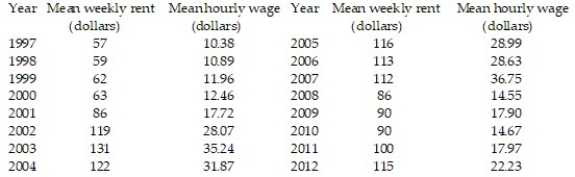 Summary statistics yield:
  = 1222.2771,
  = 3031.7125,
  = 9144.9375,
  = 21.2675, and
  Find the least squares line that uses mean hourly wage to predict mean weekly rent. Round values to the nearest ten-thousandth.
(Essay)
4.9/5 (44)
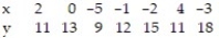
Calculate the linear correlation coefficient for the data below. 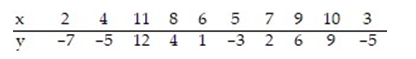
(Multiple Choice)
4.7/5 (25)
Construct a scatter diagram for the data.
-The data below are the temperatures on randomly chosen days during a summer class and the number of absences on those days. 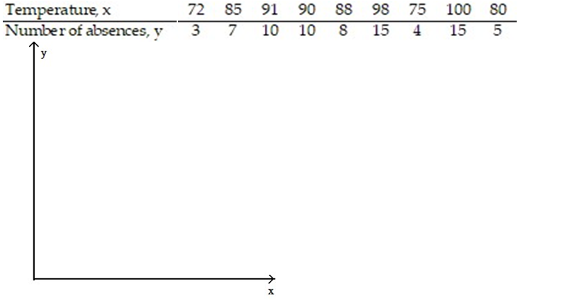
(Essay)
5.0/5 (33)
The following data represent the living situation of newlyweds in a large metropolitan area and their annual household income. What percent of people who make between $35,000 and $50,000 per year own their own home? Round to the nearest tenth of a percent. 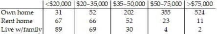
(Multiple Choice)
4.8/5 (38)
The data below are the ages and annual pharmacy b ills (in dollars) of 9 randomly selected employees. Calculate the linear correlation coefficient. 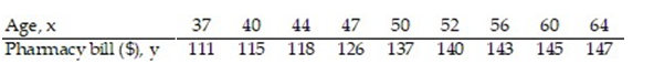
(Multiple Choice)
4.8/5 (29)
A large national bank charges local companies for using its services. A bank official reported the results of a regression analysis designed to predict the bank's charges (y), measured in dollars per month, for services rendered to local companies. One independent variable used to predict service charge to a company is the company's sales revenue (x), measured in millions of dollars. Data for 21 companies who use the bank's services were used to fit the model,  The results of the simple linear regression are provided below.
  = 2,700 + 20x, s = 65, 2-tailed p-value = 0.064 (for testing
  )Interpret the estimate of
  , the y-intercept of the line.
(Multiple Choice)
4.9/5 (29)
Make a scatter diagram for the data. Use the scatter diagram to describe how, if at all, the variables are related.
-
(Multiple Choice)
4.7/5 (30)
A real estate magazine reported the results of a regression analysis designed to predict the price (y), measured in dollars, of residential properties recently sold in a northern Virginia subdivision. One independent variable used to predict sale price is GLA, gross living area (x), measured in square feet. Data for 157 properties were used to fit the model,  =
=  +
+  x. The results of the simple linear regression are provided below.
 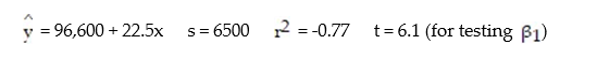 Interpret the estimate of
  , the y-intercept of the line.
(Multiple Choice)
4.8/5 (27)
Find the equation of the regression line for the given data. Round values to the nearest thousandth. 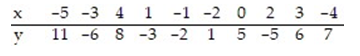
(Multiple Choice)
4.8/5 (34)
In a study of feeding behavior, zoologists recorded the number of grunts of a warthog feeding by a lake in the 15 minute period following the addition of food. The data showing the weekly number of grunts and the age of the warthog (in days) are listed below. Find and interpret the value of  . Round
  to the nearest thousandth.
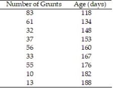
(Essay)
4.9/5 (34)
Filters
- Essay(0)
- Multiple Choice(0)
- Short Answer(0)
- True False(0)
- Matching(0)