Exam 4: Linear Regression With One Regressor

(Requires Calculus)Consider the following model: Yi = β1Xi + ui. Derive the OLS estimator for β1.

In a simple regression with an intercept and a single explanatory variable,the variation in Y 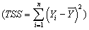can be decomposed into the explained sums of squares 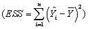and the sum of squared residuals 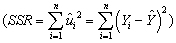(see,for example,equation (4.35)in the textbook). Consider any regression line,positively or negatively sloped in {X,Y} space.Draw a horizontal line where,hypothetically,you consider the sample mean of Y to be.Next add a single actual observation of Y. In this graph,indicate where you find the following distances: the (i)residual (ii)actual minus the mean of Y (iii)fitted value minus the mean of Y

Interpreting the intercept in a sample regression function is

The reason why estimators have a sampling distribution is that

The neoclassical growth model predicts that for identical savings rates and population growth rates,countries should converge to the per capita income level.This is referred to as the convergence hypothesis.One way to test for the presence of convergence is to compare the growth rates over time to the initial starting level. (a)If you regressed the average growth rate over a time period (1960-1990)on the initial level of per capita income,what would the sign of the slope have to be to indicate this type of convergence? Explain.Would this result confirm or reject the prediction of the neoclassical growth model? (b)The results of the regression for 104 countries were as follows: = 0.019 - 0.0006 × RelProd60 ,R2 = 0.00007,SER = 0.016, where g6090 is the average annual growth rate of GDP per worker for the 1960-1990 sample period,and RelProd60 is GDP per worker relative to the United States in 1960. Interpret the results.Is there any evidence of unconditional convergence between the countries of the world? Is this result surprising? What other concept could you think about to test for convergence between countries? (c)You decide to restrict yourself to the 24 OECD countries in the sample.This changes your regression output as follows: = 0.048 - 0.0404 RelProd60 ,R2 = 0.82 ,SER = 0.0046 How does this result affect your conclusions from above?

Assume that you have collected a sample of observations from over 100 households and their consumption and income patterns.Using these observations,you estimate the following regression Ci = β0+β1Yi+ ui where C is consumption and Y is disposable income.The estimate of β1 will tell you

At the Stock and Watson (http://www.pearsonhighered.com/stock_watson)website go to Student Resources and select the option "Datasets for Replicating Empirical Results." Then select the "California Test Score Data Used in Chapters 4-9" (caschool.xls)and open it in a spreadsheet program such as Excel. In this exercise you will estimate various statistics of the Linear Regression Model with One Regressor through construction of various sums and ratio within a spreadsheet program. Throughout this exercise,let Y correspond to Test Scores (testscore)and X to the Student Teacher Ratio (str).To generate answers to all exercises here,you will have to create seven columns and the sums of five of these.They are (i)Yi, (ii)Xi, (iii)(Yi- ), (iv)(Xi- ), (v)(Yi- )×(Xi- ), (vi)(Xi- )2, (vii)(Yi- )2 Although neither the sum of (iii)or (iv)will be required for further calculations,you may want to generate these as a check (both have to sum to zero). a.Use equation (4.7)and the sums of columns (v)and (vi)to generate the slope of the regression. b.Use equation (4.8)to generate the intercept. c.Display the regression line (4.9)and interpret the coefficients. d.Use equation (4.16)and the sum of column (vii)to calculate the regression R2. e.Use equation (4.19)to calculate the SER. f.Use the "Regression" function in Excel to verify the results.

Changing the units of measurement,e.g.measuring testscores in 100s,will do all of the following EXCEPT for changing the

In order to calculate the regression R2 you need the TSS and either the SSR or the ESS.The TSS is fairly straightforward to calculate,being just the variation of Y.However,if you had to calculate the SSR or ESS by hand (or in a spreadsheet),you would need all fitted values from the regression function and their deviations from the sample mean,or the residuals.Can you think of a quicker way to calculate the ESS simply using terms you have already used to calculate the slope coefficient?

In the simple linear regression model Yi = β0 + β1Xi + ui,

(Requires Appendix material)A necessary and sufficient condition to derive the OLS estimator is that the following two conditions hold: = 0 and = 0.Show that these conditions imply that = 0.

For the simple regression model of Chapter 4,you have been given the following data: = 274,745.75; = 8,248.979; = 5,392,705; = 163,513.03; = 179,878,841.13 (a)Calculate the regression slope and the intercept. (b)Calculate the regression R2

At the Stock and Watson (http://www.pearsonhighered.com/stock_watson)website,go to Student Resources and select the option "Datasets for Replicating Empirical Results." Then select the "California Test Score Data Used in Chapters 4-9" and read the data either into Excel or STATA (or another statistical program). Run a regression of the average reading score (read_scr)on the average math score (math_scr).What values for the slope and the intercept would you expect? Interpret the coefficients in the resulting regression output and the regression R2.

In 2001,the Arizona Diamondbacks defeated the New York Yankees in the Baseball World Series in 7 games.Some players,such as Bautista and Finley for the Diamondbacks,had a substantially higher batting average during the World Series than during the regular season.Others,such as Brosius and Jeter for the Yankees,did substantially poorer.You set out to investigate whether or not the regular season batting average is a good indicator for the World Series batting average.The results for 11 players who had the most at bats for the two teams are: = -0.347 + 2.290 AZSeasavg ,R2=0.11,SER = 0.145, = 0.134 + 0.136 NYSeasavg ,R2=0.001,SER = 0.092, where Wsavg and Seasavg indicate the batting average during the World Series and the regular season respectively. (a)Focusing on the coefficients first,what is your interpretation? (b)What can you say about the explanatory power of your equation? What do you conclude from this?

To decide whether the slope coefficient indicates a "large" effect of X on Y,you look at the

The following are all least squares assumptions with the exception of:

(Requires Appendix)The sample regression line estimated by OLS

The slope estimator,β1,has a smaller standard error,other things equal,if

The standard error of the regression (SER)is defined as follows

The OLS residuals, i,are sample counterparts of the population