Exam 14: Introduction to Time Series Regression and Forecasting
Exam 1: Economic Questions and Data17 Questions
Exam 2: Review of Probability71 Questions
Exam 3: Review of Statistics63 Questions
Exam 4: Linear Regression With One Regressor65 Questions
Exam 5: Regression With a Single Regressor: Hypothesis Tests and Confidence Intervals59 Questions
Exam 6: Linear Regression With Multiple Regressors65 Questions
Exam 7: Hypothesis Tests and Confidence Intervals in Multiple Regression65 Questions
Exam 8: Nonlinear Regression Functions62 Questions
Exam 9: Assessing Studies Based on Multiple Regression65 Questions
Exam 10: Regression With Panel Data50 Questions
Exam 11: Regression With a Binary Dependent Variable50 Questions
Exam 12: Instrumental Variables Regression50 Questions
Exam 13: Experiments and Quasi-Experiments50 Questions
Exam 14: Introduction to Time Series Regression and Forecasting50 Questions
Exam 15: Estimation of Dynamic Causal Effects50 Questions
Exam 16: Additional Topics in Time Series Regression50 Questions
Exam 17: The Theory of Linear Regression With One Regressor49 Questions
Exam 18: The Theory of Multiple Regression50 Questions
Select questions type
Consider the standard AR(1)Yt = β0 + β1Yt-1 + ut,where the usual assumptions hold.
(a)Show that yt = β0Yt-1 + ut,where yt is Yt with the mean removed,i.e. ,yt = Yt - E(Yt).Show that E(Yt)= 0.
(b)Show that the r-period ahead forecast E(  +r
+r  )=
)= 
 .If 0 < β1 < 1,how does the r-period ahead forecast behave as r becomes large? What is the forecast of
  for large r?
(c)The median lag is the number of periods it takes a time series with zero mean to halve its current value (in expectation),i.e. ,the solution r to E(
for large r?
(c)The median lag is the number of periods it takes a time series with zero mean to halve its current value (in expectation),i.e. ,the solution r to E(  +r
+r  )= 0.5
  .Show that in the present case this is given by r = -
  .
.
(Essay)
4.9/5  (43)
(43)
If a "break" occurs in the population regression function,then
(Multiple Choice)
4.8/5 (37)
You collect monthly data on the money supply (M2)for the United States from 1962:1-2002:4 to forecast future money supply behavior. 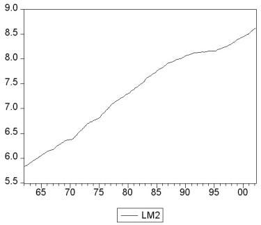
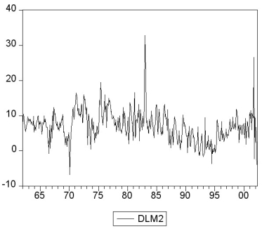 where LM2 and DLM2 are the log level and growth rate of M2.
(a)Using quarterly data,when analyzing inflation and unemployment in the United States,the textbook converted log levels of variables into growth rates by differencing the log levels,and then multiplying these by 400.Given that you have monthly data,how would you proceed here?
(b)How would you go about testing for a stochastic trend in LM2 and DLM2? Be specific about how to decide the number of lags to be included and whether or not to include a deterministic trend in your test.The textbook found the (quarterly)inflation rate to have a unit root.Does this have any affect on your expectation about whether or not the (monthly)money growth rate should be stationary?
(c)You decide to conduct an ADF unit root test for LM2,DLM2,and the change in the growth rate ΔDLM2.This results in the following t-statistic on the parameter of interest.
where LM2 and DLM2 are the log level and growth rate of M2.
(a)Using quarterly data,when analyzing inflation and unemployment in the United States,the textbook converted log levels of variables into growth rates by differencing the log levels,and then multiplying these by 400.Given that you have monthly data,how would you proceed here?
(b)How would you go about testing for a stochastic trend in LM2 and DLM2? Be specific about how to decide the number of lags to be included and whether or not to include a deterministic trend in your test.The textbook found the (quarterly)inflation rate to have a unit root.Does this have any affect on your expectation about whether or not the (monthly)money growth rate should be stationary?
(c)You decide to conduct an ADF unit root test for LM2,DLM2,and the change in the growth rate ΔDLM2.This results in the following t-statistic on the parameter of interest.
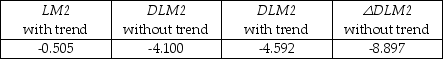 Find the critical value at the 1%,5%,and 10% level and decide which of the coefficients is significant.What is the alternative hypothesis?
(d)In forecasting the money growth rate,you add lags of the monetary base growth rate (DLMB)to see if you can improve on the forecasting performance of a chosen AR(10)model in DLM2.You perform a Granger causality test on the 9 lags of DLMB and find a F-statistic of 2.31.Discuss the implications.
(e)Curious about the result in the previous question,you decide to estimate an ADL(10,10)for DLMB and calculate the F-statistic for the Granger causality test on the 9 lag coefficients of DLM2.This turns out to be 0.66.Discuss.
(f)Is there any a priori reason for you to be skeptical of the results? What other tests should you perform?
Find the critical value at the 1%,5%,and 10% level and decide which of the coefficients is significant.What is the alternative hypothesis?
(d)In forecasting the money growth rate,you add lags of the monetary base growth rate (DLMB)to see if you can improve on the forecasting performance of a chosen AR(10)model in DLM2.You perform a Granger causality test on the 9 lags of DLMB and find a F-statistic of 2.31.Discuss the implications.
(e)Curious about the result in the previous question,you decide to estimate an ADL(10,10)for DLMB and calculate the F-statistic for the Granger causality test on the 9 lag coefficients of DLM2.This turns out to be 0.66.Discuss.
(f)Is there any a priori reason for you to be skeptical of the results? What other tests should you perform?
(Essay)
4.8/5 (36)
One reason for computing the logarithms (ln),or changes in logarithms,of economic time series is that
(Multiple Choice)
4.7/5 (45)
Problems caused by stochastic trends include all of the following with the exception of
(Multiple Choice)
4.9/5 (36)
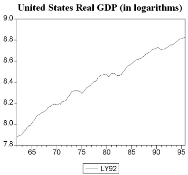
The following two graphs give you a plot of the United States aggregate unemployment rate for the sample period 1962:I to 1999:IV,and the (log)level of real United States GDP for the sample period 1962:I to 1995:IV.You want test for stationarity in both cases.Indicate whether or not you should include a time trend in your Augmented Dickey-Fuller test and why. 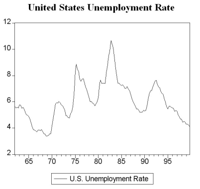
(Essay)
4.9/5 (32)
You have collected data for real GDP (Y)and have estimated the following function:
ln  t = 7.866 + 0.00679×Zeit
(0.007)(0.00008)
t = 1961:I - 2007:IV,R2 = 0.98,SER = 0.036
where Zeit is a deterministic time trend,which takes on the value of 1 during the first quarter of 1961,and is increased by one for each following quarter.
a.Interpret the slope coefficient.Does it make sense?
b.Interpret the regression R2.Are you impressed by its value?
c.Do you think that given the regression R2,you should use the equation to forecast real GDP beyond the sample period?
t = 7.866 + 0.00679×Zeit
(0.007)(0.00008)
t = 1961:I - 2007:IV,R2 = 0.98,SER = 0.036
where Zeit is a deterministic time trend,which takes on the value of 1 during the first quarter of 1961,and is increased by one for each following quarter.
a.Interpret the slope coefficient.Does it make sense?
b.Interpret the regression R2.Are you impressed by its value?
c.Do you think that given the regression R2,you should use the equation to forecast real GDP beyond the sample period?
(Essay)
4.9/5 (31)
The textbook displayed the accompanying four economic time series with "markedly different patterns." For each indicate what you think the sample autocorrelations of the level (Y)and change (△Y)will be and explain your reasoning.
(a)  (b)
(b) 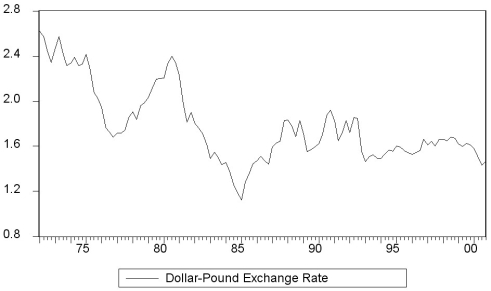 (c)
(c) 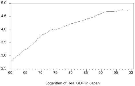 (d)
(d) 
(Essay)
4.9/5 (27)
One of the sources of error in the RMSFE in the AR(1)model is
(Multiple Choice)
4.8/5 (38)
(Requires Internet Access for the test question)
The following question requires you to download data from the internet and to load it into a statistical package such as STATA or EViews.
a.Your textbook estimates an AR(1)model (equation 14.7)for the change in the inflation rate using a sample period 1962:I - 2004:IV.Go to the Stock and Watson companion website for the textbook and download the data "Macroeconomic Data Used in Chapters 14 and 16." Enter the data for consumer price index,calculate the inflation rate,the acceleration of the inflation rate,and replicate the result on page 526 of your textbook.Make sure to use heteroskedasticity-robust standard error option for the estimation.
b.Next find a website with more recent data,such as the Federal Reserve Economic Data (FRED)site at the Federal Reserve Bank of St.Louis.Locate the data for the CPI,which will be monthly,and convert the data in quarterly averages.Then,using a sample from 1962:I - 2009:IV,re-estimate the above specification and comment on the changes that have occurred.
c.Based on the BIC,how many lags should be included in the forecasting equation for the change in the inflation rate? Use the new data set and sample period to answer the question.
(Essay)
4.9/5 (34)
You set out to forecast the unemployment rate in the United States (UrateUS),using quarterly data from 1960,first quarter,to 1999,fourth quarter.
(a)The following table presents the first four autocorrelations for the United States aggregate unemployment rate and its change for the time period 1960 (first quarter)to 1999 (fourth quarter).Explain briefly what these two autocorrelations measure.
First Four Autocorrelations of the U.S.Unemployment Rate and Its Change,
1960:I - 1999:IV
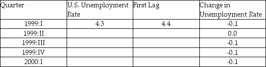
 (b)The accompanying table gives changes in the United States aggregate unemployment rate for the period 1999:I-2000:I and levels of the current and lagged unemployment rates for 1999:I.Fill in the blanks for the missing unemployment rate levels.
Changes in Unemployment Rates in the United States
First Quarter 1999 to First Quarter 2000
(b)The accompanying table gives changes in the United States aggregate unemployment rate for the period 1999:I-2000:I and levels of the current and lagged unemployment rates for 1999:I.Fill in the blanks for the missing unemployment rate levels.
Changes in Unemployment Rates in the United States
First Quarter 1999 to First Quarter 2000
 (c)You decide to estimate an AR(1)in the change in the United States unemployment rate to forecast the aggregate unemployment rate.The result is as follows:
  = -0.003 + 0.621 △ UrateUSt-1,R2 = 0.393,SER = 0.255
(0.022)(0.106)
The AR(1)coefficient for the change in the inflation rate was 0.211 and the regression R2 was 0.04.What does the difference in the results suggest here?
(d)The textbook used the change in the log of the price level to approximate the inflation rate,and then predicted the change in the inflation rate.Why aren't logarithms used here?
(e)If much of the forecast error arises as a result of future error terms dominating the error resulting from estimating the unknown coefficients,then what is your best guess of the RMSFE here?
(f)The actual unemployment rate during the fourth quarter of 1999 is 4.1 percent,and it decreased from the third quarter to the fourth quarter by 0.1 percent.What is your forecast for the unemployment rate level in the first quarter of 1996?
(g)You want to see how sensitive your forecast is to changes in the specification.Given that you have estimated the regression with quarterly data,you consider an AR(4)model.This results in the following output
= -0.003 + 0.621 △ UrateUSt-1,R2 = 0.393,SER = 0.255
(0.022)(0.106)
The AR(1)coefficient for the change in the inflation rate was 0.211 and the regression R2 was 0.04.What does the difference in the results suggest here?
(d)The textbook used the change in the log of the price level to approximate the inflation rate,and then predicted the change in the inflation rate.Why aren't logarithms used here?
(e)If much of the forecast error arises as a result of future error terms dominating the error resulting from estimating the unknown coefficients,then what is your best guess of the RMSFE here?
(f)The actual unemployment rate during the fourth quarter of 1999 is 4.1 percent,and it decreased from the third quarter to the fourth quarter by 0.1 percent.What is your forecast for the unemployment rate level in the first quarter of 1996?
(g)You want to see how sensitive your forecast is to changes in the specification.Given that you have estimated the regression with quarterly data,you consider an AR(4)model.This results in the following output  = -0.005 + 0.663 △UrateUSt-1 - 0.082 UrateUSt-2
(0.022)(0.125)(0.139)
+ 0.106 UrateUSt-3 - 0.176 △ UrateUSt-4 ,R2 = 0.416,SER = 0.253
(0.117)(0.091)
What is your forecast for the unemployment rate level in 2000:I? Compare the forecast error of the AR(4)model with the forecast error of the AR(1)model.
(h)There does not seem to be much difference in the forecast of the unemployment rate level,whether you use the AR(1)or the AR(4).Given the various information criteria and the regression R2 below,which model should you use for forecasting?
p BIC AIC R2
0 0.604 0.624 0.000
1 0.158 0.1181 0.393
2 0.185 0.125 0.397
3 0.217 0.138 0.400
4 0.218 0.1183 0.416
5 0.249 0.130 0.417
6 0.277 0.138 0.420
= -0.005 + 0.663 △UrateUSt-1 - 0.082 UrateUSt-2
(0.022)(0.125)(0.139)
+ 0.106 UrateUSt-3 - 0.176 △ UrateUSt-4 ,R2 = 0.416,SER = 0.253
(0.117)(0.091)
What is your forecast for the unemployment rate level in 2000:I? Compare the forecast error of the AR(4)model with the forecast error of the AR(1)model.
(h)There does not seem to be much difference in the forecast of the unemployment rate level,whether you use the AR(1)or the AR(4).Given the various information criteria and the regression R2 below,which model should you use for forecasting?
p BIC AIC R2
0 0.604 0.624 0.000
1 0.158 0.1181 0.393
2 0.185 0.125 0.397
3 0.217 0.138 0.400
4 0.218 0.1183 0.416
5 0.249 0.130 0.417
6 0.277 0.138 0.420
(Essay)
5.0/5 (41)
Having learned in macroeconomics that consumption depends on disposable income,you want to determine whether or not disposable income helps predict future consumption.You collect data for the sample period 1962:I to 1995:IV and plot the two variables.
(a)To determine whether or not past values of personal disposable income growth rates help to predict consumption growth rates,you estimate the following relationship.  t = 1.695 + 0.126 ΔLnCt-1 + 0.153 ΔLnCt-2,
(0.484)(0.099)(0.103)
+ 0.294 ΔLnCt-3 - 0.008 ΔLnCt-4
(0.103)(0.102)
+ 0.088 ΔLnYt-1 - 0.031 ΔLnYt-2 - 0.050 ΔLnYt-3 - 0.091 ΔLnYt-4
(0.076)(0.078)(0.078)(0.074)
The Granger causality test for the exclusion on all four lags of the GDP growth rate is 0.98.Find the critical value for the 1%,the 5%,and the 10% level from the relevant table and make a decision on whether or not these additional variables Granger cause the change in the growth rate of consumption.
(b)You are somewhat surprised about the result in the previous question and wonder,how sensitive it is with regard to the lag length in the ADL(p,q)model.As a result,you calculate BIC and AIC of p and q from 0 to 6.The results are displayed in the accompanying table:
t = 1.695 + 0.126 ΔLnCt-1 + 0.153 ΔLnCt-2,
(0.484)(0.099)(0.103)
+ 0.294 ΔLnCt-3 - 0.008 ΔLnCt-4
(0.103)(0.102)
+ 0.088 ΔLnYt-1 - 0.031 ΔLnYt-2 - 0.050 ΔLnYt-3 - 0.091 ΔLnYt-4
(0.076)(0.078)(0.078)(0.074)
The Granger causality test for the exclusion on all four lags of the GDP growth rate is 0.98.Find the critical value for the 1%,the 5%,and the 10% level from the relevant table and make a decision on whether or not these additional variables Granger cause the change in the growth rate of consumption.
(b)You are somewhat surprised about the result in the previous question and wonder,how sensitive it is with regard to the lag length in the ADL(p,q)model.As a result,you calculate BIC and AIC of p and q from 0 to 6.The results are displayed in the accompanying table:
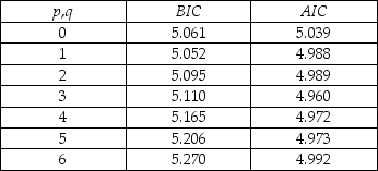 Which values for p and q should you choose?
(c)Estimating an ADL(1,1)model gives you a t-statistic of 1.28 on the coefficient of lagged disposable income growth.What does the Granger causality test suggest about the inclusion of lagged income growth as a predictor of consumption growth?
Which values for p and q should you choose?
(c)Estimating an ADL(1,1)model gives you a t-statistic of 1.28 on the coefficient of lagged disposable income growth.What does the Granger causality test suggest about the inclusion of lagged income growth as a predictor of consumption growth?
(Essay)
4.8/5 (29)
The time interval between observations can be all of the following with the exception of data collected
(Multiple Choice)
4.8/5 (28)
Filters
- Essay(0)
- Multiple Choice(0)
- Short Answer(0)
- True False(0)
- Matching(0)