Exam 13: Multiple Regression Analysis
Exam 1: Describing Data With Graphs134 Questions
Exam 2: Describing Data With Numerical Measures235 Questions
Exam 3: Describing Bivariate Data57 Questions
Exam 4: A: probability and Probability Distributions107 Questions
Exam 4: B: probability and Probability Distributions157 Questions
Exam 5: Several Useful Discrete Distributions166 Questions
Exam 6: The Normal Probability Distribution235 Questions
Exam 7: Sampling Distributions231 Questions
Exam 8: Large-Sample Estimation187 Questions
Exam 9: A: large-Sample Tests of Hypotheses154 Questions
Exam 9: B: large-Sample Tests of Hypotheses106 Questions
Exam 10: A: Inference From Small Samples192 Questions
Exam 10: B: Inference From Small Samples124 Questions
Exam 11: A: The Analysis of Variance136 Questions
Exam 11: B: The Analysis of Variance137 Questions
Exam 12: A: linear Regression and Correlation131 Questions
Exam 12: B: linear Regression and Correlation171 Questions
Exam 13: Multiple Regression Analysis232 Questions
Exam 14: Analysis of Categorical Data158 Questions
Exam 15: A:nonparametric Statistics139 Questions
Exam 15: B:nonparametric Statistics95 Questions
Select questions type
Chemical Comparisons Narrative
A chemist was interested in examining the effects of three chemicals on a chemical process yield. Let  , i = 1, 2, 3, represent the effects of the three chemicals, respectively, and y be the process yield. The following output was generated using statistical software.
Regression Analysis
, i = 1, 2, 3, represent the effects of the three chemicals, respectively, and y be the process yield. The following output was generated using statistical software.
Regression Analysis 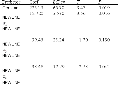 S = 14.01 R-Sq = 95.1% R-Sq(adj) = 92.1
Analysis of Variance
S = 14.01 R-Sq = 95.1% R-Sq(adj) = 92.1
Analysis of Variance  -Refer to Chemical Comparisons Narrative. Find the least squares regression equation.
(Essay)
4.9/5  (33)
(33)
In a multiple regression model, what is assumed to be true of the standard deviation of the error variable  ?
?
(Multiple Choice)
4.9/5 (40)
In a multiple regression , the regression equation is  . The estimated value for
  when
when  and
and  is 48.
(True/False)
4.7/5 (31)
Personal Spending and Personal Income
Is personal spending linearly related to orders for durable goods and personal income? A recent study reported the amounts of personal spending (in trillions of dollars), amount spent on durable goods (in billions of dollars), and personal income (in trillions of dollars). A statistical package was used to fit a linear regression model, producing the output below. 
 R2 = 95.9% R2(adj) = 95.0%, s = 0.0144 with 12 - 3 = 9 df.
-A medical study investigated the link between obesity and television viewing habits in children. One part of the study involved characterizing the difference in viewing habits between boys and girls. A regression model was used to compare the number of hours of television watched per week by boys with the number watched by girls. Use the computer printout below to determine whether there is a significant difference between these two groups. The variable named "Gender" in the printout is equal to one if the subject is female, and 0 if the subject is male. State the null and alternative hypotheses of interest. State your conclusion based on a 0.05 significance level.
The regression equation is Hours = 21.5
R2 = 95.9% R2(adj) = 95.0%, s = 0.0144 with 12 - 3 = 9 df.
-A medical study investigated the link between obesity and television viewing habits in children. One part of the study involved characterizing the difference in viewing habits between boys and girls. A regression model was used to compare the number of hours of television watched per week by boys with the number watched by girls. Use the computer printout below to determine whether there is a significant difference between these two groups. The variable named "Gender" in the printout is equal to one if the subject is female, and 0 if the subject is male. State the null and alternative hypotheses of interest. State your conclusion based on a 0.05 significance level.
The regression equation is Hours = 21.5  0.201 Gender
  Analysis of Variance
(Essay)
4.7/5 (37)
The larger the value of the coefficient of multiple determination  the larger the value of the F-test statistic that is used for testing the usefulness of the multiple regression model.
(True/False)
4.9/5 (31)
In a multiple regression model, if the residuals have a constant variance, which of the following should be evident?
(Multiple Choice)
4.8/5 (33)
Which of the following is the correct interpretation of the multiple-regression equation 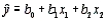 ?
?
(Multiple Choice)
4.7/5 (34)
Life Expectancy Narrative
An actuary wanted to develop a model to predict how long individuals will live. After consulting a number of physicians, she collected the age at death (y), the average number of hours of exercise per week (  ), the cholesterol level (
  ), and the number of points that the individual's blood pressure exceeded the recommended value (
  ). A random sample of 40 individuals was selected. The computer output of the multiple regression model is shown below.
The regression equation is
). A random sample of 40 individuals was selected. The computer output of the multiple regression model is shown below.
The regression equation is 
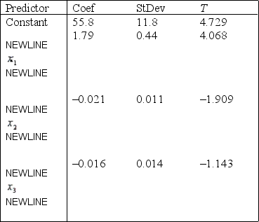 S = 9.47 R-Sq = 22.5%
Analysis of Variance
S = 9.47 R-Sq = 22.5%
Analysis of Variance  -Refer to Life Expectancy Narrative. Interpret the coefficient
  .
.
(Essay)
4.9/5 (39)
In regression analysis, to what does the term "multicollinearity" refer?
(Multiple Choice)
4.7/5 (34)
A multiple regression equation includes five predictor variables, and the coefficient of multiple determination is 0.7921. The percentage of the variation in  that is explained by the regression equation is 89%.
(True/False)
4.8/5 (31)
For each x term in the multiple regression equation, the corresponding  is referred to as a partial regression coefficient.
(True/False)
4.8/5 (31)
In order to test the validity of a multiple regression model involving 5 independent variables and 30 observations, what are the respective numerator and denominator degrees of freedom for the critical value of F?
(Multiple Choice)
4.8/5 (38)
Suppose that you fit the model 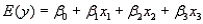 to 15 data points and found F equal to 52.36.
a. Do the data provide sufficient evidence to indicate that the model contributes information for the prediction of y? Test using a 5% level of significance.
b. Use the value of F to calculate
to 15 data points and found F equal to 52.36.
a. Do the data provide sufficient evidence to indicate that the model contributes information for the prediction of y? Test using a 5% level of significance.
b. Use the value of F to calculate  Interpret its value.
(Essay)
4.8/5 (35)
In a multiple regression model, the mean of the residuals is equal to the variance of all combinations of levels of the independent variables.
(True/False)
4.9/5 (32)
Electric Usage Narrative
The power company claims the amount of electricity used by a house (y) depends on  = square metres of heated space,
  = mean outside temperature, and
  = mean hours of sunlight per day. Partial statistical software output is given below.
Regression Analysis
The regression equation is = 357 + 0.808
= mean hours of sunlight per day. Partial statistical software output is given below.
Regression Analysis
The regression equation is = 357 + 0.808  - 16.6
  + 40
+ 40 
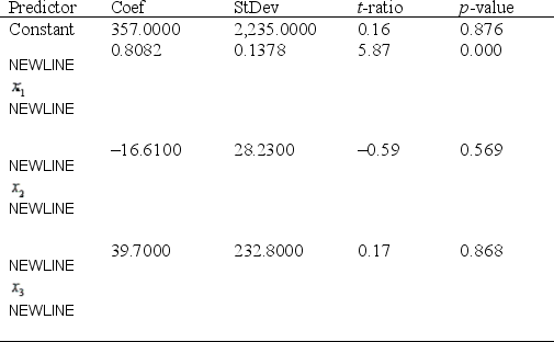 S = 267.7 R-sq = 82.0% R-sq(adj) = 76.6%
Analysis of Variance
S = 267.7 R-sq = 82.0% R-sq(adj) = 76.6%
Analysis of Variance  -Refer to Electric Usage Narrative. Does the regression model appear to be useful? Justify your answer. (Use
  = 0.05.)
(Essay)
4.8/5 (30)
In order to incorporate qualitative variables into a regression model, one or more dummy variables are needed.
(True/False)
4.8/5 (28)
What may be deduced if multicollinearity exists among the independent variables included in a multiple regression model?
(Multiple Choice)
4.8/5 (37)
Demographic Variables and TV Narrative
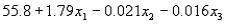
A statistician wanted to determine if the demographic variables of age, education, and income influence the number of hours of television watched per week. A random sample of 25 adults was selected to estimate the multiple regression model: 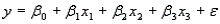 , where y is the number of hours of television watched last week,
  is the age (in years),
  is the number of years of education, and
  is income (in $1000s). The computer output is shown below.
The regression equation is
is income (in $1000s). The computer output is shown below.
The regression equation is 
 S = 4.51 R-Sq = 34.8%
Analysis of Variance
S = 4.51 R-Sq = 34.8%
Analysis of Variance  -Refer to Eating Habits of Canadians. Write the equations of the two straight lines that describe the trend in consumption over the period of 30 years for beef and for chicken.
(Essay)
4.9/5 (37)
Multicollinearity will result in excessively low standard errors of the parameter estimates reported in the regression output.
(True/False)
4.9/5 (31)
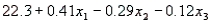
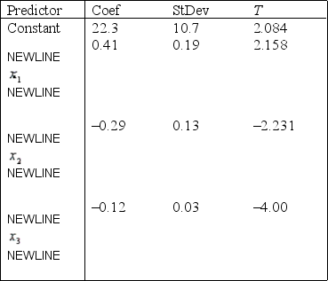
Use the following partial output and residual plot generated using statistical software to determine whether there are any potential outliers in this data. 
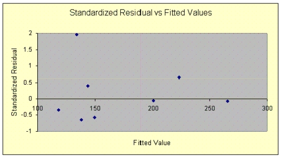
(Essay)
4.8/5 (26)
Filters
- Essay(0)
- Multiple Choice(0)
- Short Answer(0)
- True False(0)
- Matching(0)