Exam 13: Multiple Regression Analysis

An adjusted coefficient of multiple determination, denoted by (adj), is adjusted for the degrees of freedom.

The two largest values in a correlation matrix are the 0.89 correlation between y and and the 0.83 correlation between y and . During a stepwise regression analysis, is the first independent variable brought into the equation. Will necessarily be next? If not, why not?

To test the validity of a multiple regression model, which of the following tests do we use for the null hypothesis that the regression coefficients are all 0?

An estimated partial-regression coefficient gives the partial change in y for a unit change in that independent variable, while holding other independent variables constant.

A multiple regression model involves 3 predictor variables and a sample of 20 data points. If we want to test the usefulness of the model at the 1% significance level, what is the critical value of the rejection region?

In order to test the validity of a multiple regression model involving 4 predictor variables and 25 observations, what are the numerator and denominator degrees of freedom ( , respectively) for the critical value of F?

College Textbook Sales Narrative A publisher of college textbooks conducted a study to relate profit per text y to cost of sales x over a six-year period when its sales force (and sales costs) were growing rapidly. These inflation-adjusted data (in thousands of dollars) were collected: Expecting profit per book to rise and then plateau, the publisher fitted the model 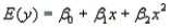to the data. -Refer to College Textbook Sales Narrative. How much of the regression sum of squares is accounted for by the quadratic term? By the linear term?

Air Pollution Monitors Narrative An experiment was designed to compare several different types of air pollution monitors. Each monitor was set up and then exposed to different concentrations of ozone, ranging between 15 and 230 parts per million (ppm), for periods of 8-72 hours. Filters on the monitor were then analyzed, and the response of the monitor was measured. The results for one type of monitor showed a linear pattern. The results for another type of monitor are listed in the table. -Refer to Air Pollution Monitors Narrative. Find on the printout. What does this value tell you about the effectiveness of the multiple regression analysis?

Life Expectancy Narrative An actuary wanted to develop a model to predict how long individuals will live. After consulting a number of physicians, she collected the age at death (y), the average number of hours of exercise per week ( ), the cholesterol level ( ), and the number of points that the individual's blood pressure exceeded the recommended value ( ). A random sample of 40 individuals was selected. The computer output of the multiple regression model is shown below. 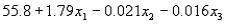The regression equation is S = 9.47 R-Sq = 22.5% Analysis of Variance -Refer to Life Expectancy Narrative. Is there sufficient evidence at the 5% significance level to infer that the number of points that the individual's blood pressure exceeded the recommended value and the age at death are negatively linearly related? Justify your conclusion.

Qualitative predictor variables are entered into a regression model through dummy variables.

A multiple regression analysis includes 25 data points and 4 independent variables, and produces SST = 400 and SSR = 300. Then, the multiple standard error of estimate is 5.

Demographic Variables and TV Narrative A statistician wanted to determine if the demographic variables of age, education, and income influence the number of hours of television watched per week. A random sample of 25 adults was selected to estimate the multiple regression model: , where y is the number of hours of television watched last week, is the age (in years), is the number of years of education, and is income (in $1000s). The computer output is shown below. 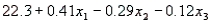The regression equation is S = 4.51 R-Sq = 34.8% Analysis of Variance -Refer to Eating Habits of Canadians. How well does the model fit? Use any relevant statistics and diagnostic tools from the printout to answer this question.

In a regression setting, if you add a predictor variable to an existing model, the value of will either remain the same or increase. However, in selecting a model, you should consider the value of the adjusted as well as .

In constructing a multiple regression model with two independent variables and it was known that the correlation between and y is 0.75, and the correlation between and y is 0.55. Based on this information, the regression model containing both independent variables will explain 65% of the variation in the dependent variable y.

Air Pollution Monitors Narrative An experiment was designed to compare several different types of air pollution monitors. Each monitor was set up and then exposed to different concentrations of ozone, ranging between 15 and 230 parts per million (ppm), for periods of 8-72 hours. Filters on the monitor were then analyzed, and the response of the monitor was measured. The results for one type of monitor showed a linear pattern. The results for another type of monitor are listed in the table. -Refer to Air Pollution Monitors Narrative. Plot the data. What model would you expect to provide the best fit to the data? Write the equation of that model.

Suppose that one equation has three explanatory variables and an F-ratio of 52. Another equation has five explanatory variables and an F-ratio of 40. The first equation will always be considered a better model.

Having a large number of predictors in a regression model guarantees that the model fit is good.

When multicollinearity is present, the estimated regression coefficients will have large standard error, causing imprecision in confidence and prediction intervals.

When a stepwise procedure is used, a variable selected at an earlier step can be removed from the model if, in the presence of other variables, it no longer contributes significantly to explaining the variation in the dependent variable y.

In a simple linear regression , the following pairs of ( ) are given: (6.75, 7.42), (8.96, 8.06), (10.30, 11.65), and (13.24, 12.15). Which of these values is equal to the sum of squares for error?