Exam 13: Multiple Regression Analysis
Exam 1: Describing Data With Graphs134 Questions
Exam 2: Describing Data With Numerical Measures235 Questions
Exam 3: Describing Bivariate Data57 Questions
Exam 4: A: probability and Probability Distributions107 Questions
Exam 4: B: probability and Probability Distributions157 Questions
Exam 5: Several Useful Discrete Distributions166 Questions
Exam 6: The Normal Probability Distribution235 Questions
Exam 7: Sampling Distributions231 Questions
Exam 8: Large-Sample Estimation187 Questions
Exam 9: A: large-Sample Tests of Hypotheses154 Questions
Exam 9: B: large-Sample Tests of Hypotheses106 Questions
Exam 10: A: Inference From Small Samples192 Questions
Exam 10: B: Inference From Small Samples124 Questions
Exam 11: A: The Analysis of Variance136 Questions
Exam 11: B: The Analysis of Variance137 Questions
Exam 12: A: linear Regression and Correlation131 Questions
Exam 12: B: linear Regression and Correlation171 Questions
Exam 13: Multiple Regression Analysis232 Questions
Exam 14: Analysis of Categorical Data158 Questions
Exam 15: A:nonparametric Statistics139 Questions
Exam 15: B:nonparametric Statistics95 Questions
Select questions type
The adjusted value of  is used mainly to compare two or more regression models that have the same number of independent predictors to determine which one fits the data better.
(True/False)
4.8/5  (32)
(32)
In a multiple regression model, adding more independent variables that have a low correlation with the dependent variable will decrease the value of the coefficient of multiple determination.
(True/False)
4.7/5 (33)
Electric Usage Narrative
The power company claims the amount of electricity used by a house (y) depends on  = square metres of heated space,
  = mean outside temperature, and
  = mean hours of sunlight per day. Partial statistical software output is given below.
Regression Analysis
The regression equation is = 357 + 0.808
= mean hours of sunlight per day. Partial statistical software output is given below.
Regression Analysis
The regression equation is = 357 + 0.808  - 16.6
  + 40
+ 40 
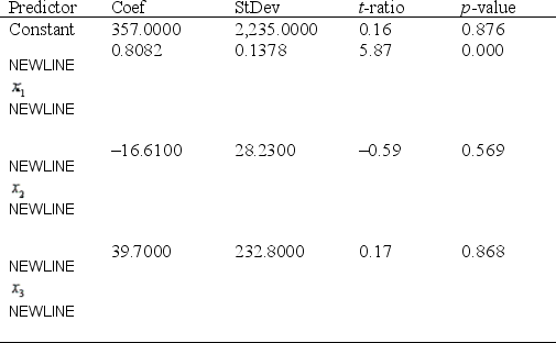 S = 267.7 R-sq = 82.0% R-sq(adj) = 76.6%
Analysis of Variance
S = 267.7 R-sq = 82.0% R-sq(adj) = 76.6%
Analysis of Variance  -Refer to Electric Usage Narrative. Construct a 99% confidence interval for
  .
.
(Essay)
4.8/5 (29)
A multiple regression model forms a plane through multidimensional space.
(True/False)
4.8/5 (37)
Assume that a company is tracking its advertising expenditures as they relate to television (  ) and radio advertising (
  ). The owner of the company believes that it would improve the regression model to add a third variable that represents the sum of the advertising on radio and television (
  =
=  +
+  ). This assessment is generally correct.
(True/False)
4.9/5 (25)
A coefficient of multiple correlation is a measure of how well an estimated regression plane (or hyperplane) fits the sample data on which it is based.
(True/False)
4.9/5 (39)
One of the consequences of multicollinearity in multiple regression is inflated standard errors in some or all of the estimated slope coefficients.
(True/False)
4.9/5 (33)
What is stepwise regression, and when is it desirable to make use of this multiple regression technique?
(Essay)
4.9/5 (24)
Demographic Variables and TV Narrative
A statistician wanted to determine if the demographic variables of age, education, and income influence the number of hours of television watched per week. A random sample of 25 adults was selected to estimate the multiple regression model: 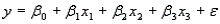 , where y is the number of hours of television watched last week,
  is the age (in years),
  is the number of years of education, and
  is income (in $1000s). The computer output is shown below.
The regression equation is
is income (in $1000s). The computer output is shown below.
The regression equation is 
 S = 4.51 R-Sq = 34.8%
Analysis of Variance
S = 4.51 R-Sq = 34.8%
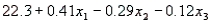
Analysis of Variance  -Refer to Eating Habits of Canadians. Use the prediction equation to find a point estimate of the average beef consumption per family of three in 2005. Compare this value with the value labelled "Fit" in the printout.
(Essay)
4.8/5 (34)
Demographic Variables and TV Narrative
A statistician wanted to determine if the demographic variables of age, education, and income influence the number of hours of television watched per week. A random sample of 25 adults was selected to estimate the multiple regression model: , where y is the number of hours of television watched last week, is the age (in years), is the number of years of education, and is income (in $1000s). The computer output is shown below.
The regression equation is S = 4.51 R-Sq = 34.8%
Analysis of Variance
-Refer to Demographic Variables and TV Narrative. Is there sufficient evidence at the 1% significance level to indicate that hours of television watched and age are linearly related? Justify your conclusion.
(Essay)
4.8/5 (35)
In testing the significance of a multiple regression model in which there are three independent variables, the null hypothesis is 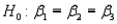 .
.
(True/False)
4.9/5 (33)
College Textbook Sales Narrative
A publisher of college textbooks conducted a study to relate profit per text y to cost of sales x over a six-year period when its sales force (and sales costs) were growing rapidly. These inflation-adjusted data (in thousands of dollars) were collected:  Expecting profit per book to rise and then plateau, the publisher fitted the model
  to the data.
-Refer to College Textbook Sales Narrative. What sign would you expect the actual value of
to the data.
-Refer to College Textbook Sales Narrative. What sign would you expect the actual value of  to have? Find the value of
  in the printout. Does this value confirm your expectation? Justify your answer.
(Essay)
4.8/5 (33)
Filters
- Essay(0)
- Multiple Choice(0)
- Short Answer(0)
- True False(0)
- Matching(0)