Exam 13: Multiple Regression Analysis

In multiple regression, a large value of the test statistic F indicates that most of the variation in y is unexplained by the regression equation and that the model is useless. A small value of F indicates that most of the variation in y is explained by the regression equation and that the model is useful.

Magazine Sales Narrative A publisher is studying the effectiveness of advertising to sell a woman's magazine. She wishes to investigate the relationship between the number of magazines sold (10,000s), the "reach" (proportion of the population who see at least one advertisement for the magazine), and the average income of the target market ($1000s). The publisher suspects people at certain income levels might be more susceptible to this advertising campaign than others. Preliminary studies show there is no evidence of a quadratic relationship between sales and either of the other two variables. Use the output below to answer the questions. The regression equation is Sales = 3.1 + 10341 Reach + 0.871 Income + 3.256 Reach*Income S = 8.43 R-sq = 82.4% Analysis of Variance -Refer to Magazine Sales Narrative. Is there an interaction effect? Test at the 5% significance level.

In order to incorporate the marital status variable into a multiple regression model, there are four possible categories for this variable: married, single, divorced, or widowed. Based on this information, four indictor variables will need to be created (one for each category) and incorporated into the regression model.

In multiple regression analysis, what does the ratio MSR/MSE equal?

Which, if any, of the following is an advantage of using stepwise regression compared to just entering all the independent variables at one time?

An estimated partial-regression coefficient is the coefficient of a dependent variable in an estimated multiple-regression equation.

Magazine Sales Narrative A publisher is studying the effectiveness of advertising to sell a woman's magazine. She wishes to investigate the relationship between the number of magazines sold (10,000s), the "reach" (proportion of the population who see at least one advertisement for the magazine), and the average income of the target market ($1000s). The publisher suspects people at certain income levels might be more susceptible to this advertising campaign than others. Preliminary studies show there is no evidence of a quadratic relationship between sales and either of the other two variables. Use the output below to answer the questions. The regression equation is Sales = 3.1 + 10341 Reach + 0.871 Income + 3.256 Reach*Income S = 8.43 R-sq = 82.4% Analysis of Variance -Refer to Magazine Sales Narrative. Write the model used for the regression.

In regression analysis, a p-value provides the probability (judged by the t-value associated with an estimated regression coefficient) of being true, given the claim The true regression coefficient equals 0.

Multicollinearity is also called collinearity and intercorrelation.

The adjusted coefficient of determination is adjusted for the number of independent variables in the model by using sum of squares rather mean squares.

Stepwise regression analysis is most useful when it is anticipated that there are curvilinear relationships between the dependent variable and the potential independent variables.

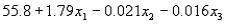
In a multiple regression involving 24 observations and 3 independent variables, the estimated regression equation is 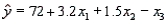. For this model, SST = 800 and SSE = 245. The value of the F statistic for testing the significance of the model is 15.102.

Life Expectancy Narrative An actuary wanted to develop a model to predict how long individuals will live. After consulting a number of physicians, she collected the age at death (y), the average number of hours of exercise per week ( ), the cholesterol level ( ), and the number of points that the individual's blood pressure exceeded the recommended value ( ). A random sample of 40 individuals was selected. The computer output of the multiple regression model is shown below. The regression equation is S = 9.47 R-Sq = 22.5% Analysis of Variance -Refer to Life Expectancy Narrative. What is the coefficient of determination? What does this statistic tell you?

In a regression model involving 40 observations, the following estimated regression model was obtained: 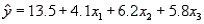. For this model, the following statistics are given: SSR = 501 and SSE = 99. What is the value of MSR?

Consider the following partial output generated using a statistical software: The regression equation is 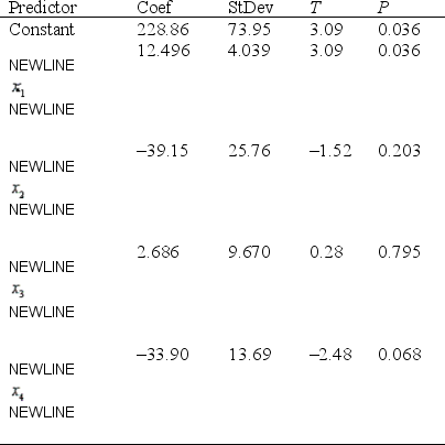S = 15.51 R-Sq = 95.2% R-Sq(adj) = 90.3% a. Which, if any, of the terms should be removed from the model first? Justify your answer. (Use a significance level of 0.05.) b. Which of the predictors makes the most significant contribution in predicting the dependent variable y? Justify your answer. c. Find and interpret the coefficient of determination.

An estimated partial-regression coefficient gives the partial change in Y for a unit change in that independent variable, while holding other independent variables constant.

In reference to the multiple regression model , if were to increase by five units, holding and constant, then the value of would decrease on average by 50 units.

The y-intercept will usually be negative in a multiple regression model when the regression slope coefficients are positive.

Personal Spending and Personal Income Is personal spending linearly related to orders for durable goods and personal income? A recent study reported the amounts of personal spending (in trillions of dollars), amount spent on durable goods (in billions of dollars), and personal income (in trillions of dollars). A statistical package was used to fit a linear regression model, producing the output below. R² = 95.9% R²(adj) = 95.0%, s = 0.0144 with 12 - 3 = 9 df. -Refer to Personal Spending and Personal Income. Use the computer output shown above to test the hypotheses vs. at the 5% significance level. What is your conclusion?

Air Pollution Monitors Narrative An experiment was designed to compare several different types of air pollution monitors. Each monitor was set up and then exposed to different concentrations of ozone, ranging between 15 and 230 parts per million (ppm), for periods of 8-72 hours. Filters on the monitor were then analyzed, and the response of the monitor was measured. The results for one type of monitor showed a linear pattern. The results for another type of monitor are listed in the table. -Refer to Air Pollution Monitors Narrative. Find the least-squares regression equation relating the monitor's response to the ozone concentration.